The VARIOGRAM Procedure

Autocorrelation Statistics Types
One measure of spatial autocorrelation provided by PROC VARIOGRAM is Moran’s  statistic, which was introduced by Moran (1950) and is defined as
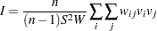 |
where 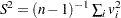 , and
, and  .
.
Another measure of spatial autocorrelation in PROC VARIOGRAM is Geary’s  statistic (Geary; 1954), defined as
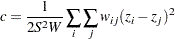 |
These expressions indicate that Moran’s coefficient makes use of the centered variable, whereas the Geary’s expression uses the noncentered values in the summation.
Inference on these two statistic types comes from approximate tests based on the asymptotic distribution of and , which both tend to a normal distribution as  increases. To this end, PROC VARIOGRAM calculates the means and variances of and . The outcome depends on the assumption made regarding the distribution
  . In particular, you can choose to investigate any of the statistics under the normality (also known as Gaussianity) or the randomization assumption. Cliff and Ord (1981) provided the equations for the means and variances of the and distributions, as described in the following.
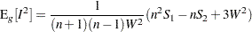
The normality assumption asserts that the random field follows a normal distribution of constant mean ( ) and variance, from which the
  values are drawn. In this case, the statistics yield
 |
and
 |
where 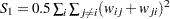 and
and 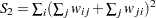 . The corresponding moments for the statistics are
 |
and
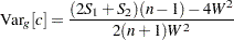 |
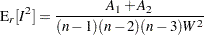
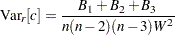
According to the randomization assumption, the and observations are considered in relation to all the different values that and could take, respectively, if the values were repeatedly randomly permuted around the domain  . The moments for the statistics are now
 |
and
 |
where  ,
,  . The factor
  is the coefficient of kurtosis that uses the sample moments
  for
for  . Finally, the statistics under the randomization assumption are given by
 |
and
 |
with  ,
,  , and
, and  .
.
If you specify LAGDISTANCE= to be larger than the maximum data distance in your domain, the binary weighting scheme used by the VARIOGRAM procedure leads to all weights  ,
,  . In this extreme case the preceding definitions can show that the variances of the and statistics become zero under either the normality or the randomization assumption.
A similar effect might occur when you have collocated observations (see the section Pair Formation). The Moran’s and Geary’s statistics allow for the inclusion of such pairs in the computations. Hence, contrary to the semivariance analysis, PROC VARIOGRAM does not exclude pairs of collocated data from the autocorrelation statistics.