The POWER Procedure
- Overview
-
Getting Started

-
Syntax
PROC POWER Statement LOGISTIC Statement MULTREG Statement ONECORR Statement ONESAMPLEFREQ Statement ONESAMPLEMEANS Statement ONEWAYANOVA Statement PAIREDFREQ Statement PAIREDMEANS Statement PLOT Statement TWOSAMPLEFREQ Statement TWOSAMPLEMEANS Statement TWOSAMPLESURVIVAL Statement TWOSAMPLEWILCOXON Statement
-
Details
Overview of Power Concepts Summary of Analyses Specifying Value Lists in Analysis Statements Sample Size Adjustment Options Error and Information Output Displayed Output ODS Table Names Computational Resources Computational Methods and Formulas ODS Graphics ODS Styles Suitable for Use with PROC POWER
-
Examples
One-Way ANOVA The Sawtooth Power Function in Proportion Analyses Simple AB/BA Crossover Designs Noninferiority Test with Lognormal Data Multiple Regression and Correlation Comparing Two Survival Curves Confidence Interval Precision Customizing Plots Binary Logistic Regression with Independent Predictors Wilcoxon-Mann-Whitney Test
- References
Analyses in the LOGISTIC Statement
Likelihood Ratio Chi-Square Test for One Predictor (TEST=LRCHI)
The power computing formula is based on Shieh and O’Brien (1998), Shieh (2000), and Self, Mauritsen, and Ohara (1992).
Define the following notation for a logistic regression analysis:
 |
 |
|||
 |
 |
|||
 |
 |
|||
 |
 |
|||
 |
 |
|||
 |
 |
|||
 |
 |
|||
 |
 |
|||
 |
 |
|||
 |
 |
|||
 |
 |
|||
 |
 |
|||
 |
 |
|||
 |
 |
|||
|
 |
|||
 |
 |
|||
 |
 |
|||
|
 |
|||
 |
 |
|||
|
|
|||
 |
 |
|||
 |
 |
|||
 |
 |
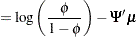
The logistic regression model is
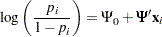 |
The hypothesis test of the first predictor variable is
 |
 |
|||
 |
 |
Assuming independence among all predictor variables,  is defined as follows:
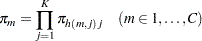 |
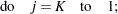
where  is calculated according to the following algorithm:
 |
|||||
 |
|||||
 |
|||||
 |
|||||
 |
|||||
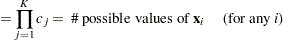
This algorithm causes the elements of the transposed vector  to vary fastest to slowest from right to left as
  increases, as shown in the following table of values:
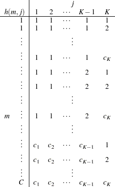 |
The  values are determined in a completely analogous manner.
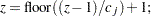
The discretization is handled as follows (unless the distribution is ordinal, or binomial with sample size parameter at least as large as requested number of bins): for  , generate
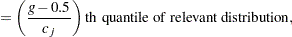
  quantiles at evenly spaced probability values such that each such quantile is at the midpoint of a bin with probability
  . In other words,
 |
 |
|||
|
 |
|||
|
 |
The primary noncentrality for the power computation is
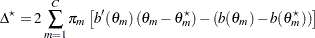 |
where
 |
 |
|||
 |
 |
|||
 |
 |
|||
 |
 |
where
 |
 |
|||
 |
 |
The power is
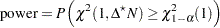 |
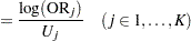
Alternative input parameterizations are handled by the following transformations:
 |
 |
|||
 |
 |