The KRIGE2D Procedure

Geometric Anisotropy

Geometric anisotropy is the simplest type of anisotropy. It occurs when the same sill (or scale) parameter is present in all directions but the range changes with direction. In geometric anisotropy the covariance model uses the same forms in all directions.

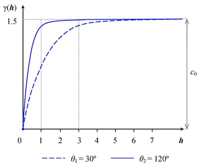
Therefore, geometric anisotropy features one single sill value, and depending on the direction the semivariogram reaches the sill within a different distance. This is illustrated in Figure 48.12, where an anisotropic exponential semivariogram is plotted. Assume that the two curves displayed in this figure have the same sill and are generated using the ranges in the direction (effective range is ) and in the direction (effective range is ).

As you can see from the figure, the ratio of the shorter to longer range is . The anisotropy factor is the value to use in the RATIO= parameter in the MODEL statement in PROC KRIGE2D. When you model geometric anisotropy . In fact, isotropy is a partial case of geometric anisotropy for which and .

Figure 48.12 Geometric Anisotropy with Major Axis in the Direction

The values of the RANGE= and ANGLE= parameters in the MODEL statement in PROC KRIGE2D are set based on the major anisotropy axis characteristics. Specifically, the RANGE= parameter is the value of the major axis range , and the ANGLE= parameter is the angle of the major axis measured clockwise from north (angles measured in this way are also known as azimuths). You can then specify the following MODEL statement in PROC KRIGE2D to approximate the covariance structure:

MODEL FORM=EXP RANGE=3 SCALE=1.5 ANGLE=30 RATIO=0.3333;

If you use a nested model, provide the type for each one of the nested structures with the FORM= option, and assign the individual SCALE= parameters so that they add up to the total sill (include in the sum the nugget effect, if present). In the typical case, all of your nested structures have the same anisotropy axes. This means that you specify the same ANGLE= parameter value for all structures. Each structure likely has its own values for the RANGE= and RATIO= parameters depending on the degree of its contribution to the nested model.

The terminology associated with geometric anisotropy is that of ellipses. To see how this comes about, consider the following hypothetical set of calculations. Let {} be a geometrically anisotropic process, and assume sufficient data points are present to calculate an experimental semivariogram at a large number of angle classes }. At each of these angles , the experimental semivariogram is plotted and the range is recorded. A diagram in polar coordinates yields an ellipse with the major axis in the direction of the largest and the minor axis perpendicular to it. For the example in Figure 48.12, the ellipse is shown in Figure 48.13(a). Its major axis has size situated at angle clockwise from north, and the minor axis has size oriented at angle clockwise from north.

The KRIGE2D procedure handles geometric anisotropy by applying a reversible transformation in two steps that converts geometric anisotropy into isotropic conditions.

The first step is to align your coordinates axes with the anisotropy ellipse axes. Specifically, you choose to rotate by an angle the standard Cartesian orientation of the coordinates system shown in Figure 48.13(a) so that the Y axis coincides with the ellipse minor axis. The rotation result is illustrated in Figure 48.13(b). The second step is to elongate the minor axis so its length equals that of the major axis of the ellipse. You can see the result in Figure 48.13(c). The computational details are shown in the following.

Figure 48.13 Transformation Applied to Geometric Anisotropy

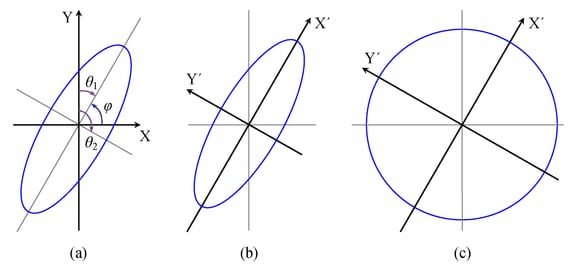
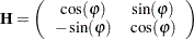
The transformation angle is measured in standard Cartesian orientation counterclockwise from the X axis (east). If the major axis azimuth is , then the Cartesian system of needs to be rotated by so that the Y axis can coincide with the ellipse minor axis; see Figure 48.13(a).

Let us call the ellipse major axis X’ and the minor axis Y’. The transformation that converts any coordinates in the system into coordinates in terms of is given by the matrix:

The elongation of the minor axis in the second step is performed with the matrix:

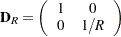Note: These two steps are sequential and their order cannot be reversed. For any point pair and with respective coordinates and in the axes, their distance is given by

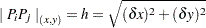where the distance components and . Based on the previous, the corresponding distances and in the coordinates system are given by the vector:

The transformed interpair distance is then:

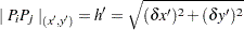As a result, the original anisotropic semivariogram in Figure 48.12 that was a function of both and is then transformed to an equivalent function only of :

This single isotropic semivariogram is then used for kriging purposes.

The two steps used by PROC KRIGE2D in the previous analysis can also be performed in a different manner. For instance, you might equivalently choose to rotate the Cartesian coordinates so that the Y axis coincides with the ellipse major axis, rather than with the minor axis as was shown earlier. Also, you might prefer to compress the major axis rather than elongating the short one. In any case, you need to perform the appropriate computations for the transformation of your choice.