Specifying the Full Measurement Model (H4) by the FACTOR Modeling Language: Lord Data
The measurement models described in the section Some Measurement Models are also known as confirmatory factor models. PROC CALIS has a specific modeling language, called FACTOR, for confirmatory factor models. You can use this modeling language for both exploratory and confirmatory factor analysis.
For example, the full measurement model H4 in the section H4: Full Measurement Model for Lord Data can be specified equivalently by the FACTOR modeling language with the following statements:
proc calis data=lord;
   factor
      F1  --->  W  X,
      F2  --->  Y  Z;
   pvar
      F1 = 1.0,
      F2 = 1.0,
      W X Y Z;
   cov
      F1 F2;
run;
In the specification, you use the FACTOR statement to invoke the FACTOR modeling language. In the FACTOR statement, you specify the paths from the latent factors to the measurement indicators. For example, F1 has two paths to its indicators, W and X. Similarly, F2 has two paths to its indicators, Y and Z. Next, you use the PVAR statement to specify the variances, which is exactly the same way you use the PATH model specification in the section H4: Full Measurement Model for Lord Data. Lastly, you use the COV statement to specify the covariance among the factors, much like you use the PCOV statement to specify the same covariance in the PATH model specification.
Given the same confirmatory factor model, there is a major difference between the paths specified by the PATH statement and the paths specified by the FACTOR statement. In the FACTOR statement, each path must start with a latent factor followed by a right arrow and the variable list. In the PATH statement, each path can start or end with an observed or latent variable, and the direction of the arrow can be left or right.
The fit summary table for the FACTOR model is shown in Figure 17.29:
Figure 17.29
Fit Summary of the Full Confirmatory Factor Model for Lord Data
| 0.7030 |
| 1 |
| 0.4018 |
| 0.0030 |
| 0.9946 |
| 0.0000 |
| 1.0000 |
This is exactly the same fit summary as shown in Figure 17.18, which is for the PATH model specification. Therefore, this confirms that the same model is being fit by the FACTOR model specification.
The estimation results are shown in Figure 17.30.
Figure 17.30
Estimation Results of Full Confirmatory Factor Model for Lord Data
| 7.5007 |
| 0.3234 |
| 23.1939 |
| [_Parm1] |
|
|
| 7.7027 |
| 0.3206 |
| 24.0235 |
| [_Parm2] |
|
|
|
| 8.5095 |
| 0.3269 |
| 26.0273 |
| [_Parm3] |
|
|
| 8.6751 |
| 0.3256 |
| 26.6430 |
| [_Parm4] |
|
|
| 0.8986 |
| 0.0186 |
| 48.1800 |
| [_Parm9] |
|
| 0.8986 |
| 0.0186 |
| 48.1800 |
| [_Parm9] |
|
|
| _Parm5 |
30.13796 |
2.47037 |
12.19979 |
| _Parm6 |
26.93217 |
2.43065 |
11.08021 |
| _Parm7 |
24.87396 |
2.35986 |
10.54044 |
| _Parm8 |
22.56264 |
2.35028 |
9.60000 |
Again, these are the same estimates as those shown in Figure 17.19, which is for the PATH model specification. The FACTOR results displayed in Figure 17.30 are arranged differently though. No paths are shown there. The relationships between the latent factors and its indicators are shown in matrix form. The factor variance and covariances are also shown in matrix form.
Specifying the Parallel Tests Model (H2) by the FACTOR Modeling Language: Lord Data
In the section H2: Two-Factor Model with Parallel Tests for Lord Data, you fit a two-factor model with parallel tests for the Lord data by the PATH modeling language in PROC CALIS. Some paths and error variance are constrained under the PATH model. You can also specify this parallel tests model by the FACTOR modeling language, as shown in the following statements:
proc calis data=lord;
   factor
      F1  --->  W  X    = 2 * beta1,
      F2  --->  Y  Z    = 2 * beta2;
   pvar
      F1  = 1.0,
      F2  = 1.0,
      W X = 2 * theta1,
      Y Z = 2 * theta2;
   cov
      F1 F2;
run;
In this specification, you specify some parameters explicitly. You apply the parameter beta1 to the loadings of both W and X on F1. This means that F1 has the same amount of effect on W and X. Similarly, you apply the parameter beta2 to the loadings of Y and Z on F2. The constraints on the error variances for W, X, Y, and Z in this FACTOR model specification are done in the same way as in the PATH model specification in the section H2: Two-Factor Model with Parallel Tests for Lord Data.
The fit summary table for this parallel tests model is shown in Figure 17.31.
Figure 17.31
Fit Summary of the Confirmatory Factor Model with Parallel Tests for Lord Data
| 1.9335 |
| 5 |
| 0.8583 |
| 0.0076 |
| 0.9970 |
| 0.0000 |
| 1.0000 |
All the fit indices shown in Figure 17.31 for the FACTOR model match the corresponding PATH model results displayed in Figure 17.24. All the estimation results in Figure 17.32 for the FACTOR model are the same as those for the corresponding PATH model in Figure 17.25.
Figure 17.32
Estimation Results of the Confirmatory Factor Model with Parallel Tests for Lord Data
| 7.6010 |
| 0.2684 |
| 28.3158 |
| [beta1] |
|
|
| 7.6010 |
| 0.2684 |
| 28.3158 |
| [beta1] |
|
|
|
| 8.5919 |
| 0.2797 |
| 30.7215 |
| [beta2] |
|
|
| 8.5919 |
| 0.2797 |
| 30.7215 |
| [beta2] |
|
|
| 0.8986 |
| 0.0187 |
| 48.1801 |
| [_Parm1] |
|
| 0.8986 |
| 0.0187 |
| 48.1801 |
| [_Parm1] |
|
|
| theta1 |
28.55545 |
1.58641 |
18.00000 |
| theta1 |
28.55545 |
1.58641 |
18.00000 |
| theta2 |
23.73200 |
1.31844 |
18.00000 |
| theta2 |
23.73200 |
1.31844 |
18.00000 |
Specifying the Parallel Tests Model (H2) by the RAM Modeling Language: Lord Data
In the preceding section, you use the FACTOR modeling language of PROC CALIS to specify the parallel tests model. This model has also been specified by the PATH modeling language in the section H2: Two-Factor Model with Parallel Tests for Lord Data. The two specifications are equivalent; they lead to the same model fitting and estimation results. The main reason for providing two different types of modeling languages in PROC CALIS is that different researchers come from different fields of applications. Some researchers might be more comfortable with the confirmatory factor tradition, and some might equate structural equation models with path diagrams for variables.
PROC CALIS has still another modeling language that is closely related to the path diagram representation: the RAM model specification. In this section, the parallel tests model (H2) described in H2: Two-Factor Model with Parallel Tests for Lord Data is used to illustrate the RAM model specification in PROC CALIS.
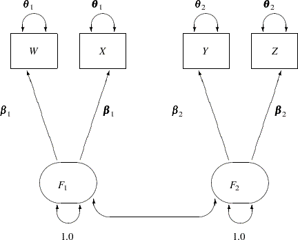
The path diagram for this model is reproduced in Figure 17.33.
The path diagram in Figure 17.33 can be readily transcribed into the RAM model specification by following these simple rules:
Each single- or double- headed path corresponds to an entry in the RAM model specification.
The single-headed paths are specified with the _A_ path type or matrix keyword.
The double-headed paths are specified with the _P_ path type or matrix keyword.
At this point, you do not need to define the RAM model matrices _A_ and _P_, as long as you recognize that they are used as keywords to distinguish different path types. There are 11 single- or double- headed paths in Figure 17.33, and therefore you expect to specify these 11 elements in the RAM model, as shown in the following statements:
proc calis data=lord;
   ram var = W X Y Z F1 F2, /* W=1, X=2, Y=3, Z=4, F1=5, F2=6*/
       _A_   1  5  beta1,
       _A_   2  5  beta1,
       _A_   3  6  beta2,
       _A_   4  6  beta2,
       _P_   5  5  1.0,
       _P_   6  6  1.0,
       _P_   1  1  theta1,
       _P_   2  2  theta1,
       _P_   3  3  theta2,
       _P_   4  4  theta2,
       _P_   5  6  ;
run;
In this specification, the RAM statement invokes the RAM modeling language. The first option is the VAR= option where you specify the variables, observed and latent, in the model. The order in the VAR= variable list represents the order of these variables in the RAM model matrices. For this example, W is 1, X is 2, and so on. Next, you specify 11 RAM entries for the 11 path elements in the path diagram shown in Figure 17.33.
The first four entries are for the single-headed paths. They all begin with the _A_ keyword. In each of these _A_ entries, you specify the variable number of the outcome variable (being pointed at), and then the variable number of the predictor variable. At the end of the entry, you can specify a parameter name, a fixed value, an initial value, or nothing. In this example, all the _A_ entries are specified with parameter names. The first two paths are constrained because they use the same parameter name beta1. The next two paths are constrained because they use the same parameter name beta2.
The rest of the RAM entries in the example are of the _P_ type, which is for the specification of variances or covariances in the RAM model (the double-headed arrows in the path diagram). The _P_ entry with [5,5] is for the variance of the fifth variable, F1, on the VAR= list. This variance is fixed at 1.0 in the model, and so is the variance of the sixth variable, F2, in the next _P_ entry.
The next four _P_ entries are for the specification of error variances of the observed variables W, X, Y, and Z. You use the desired parameter names for constraining these parameters, as required in the parallel test model.
The last _P_ entry in the RAM statement is for the covariance between the fifth variable (F1) and the sixth variable (F2). You specify neither a parameter name nor a fixed value at the end of this entry. By default, this empty parameter specification is treated as a free parameter in the model. A parameter name for this entry is generated by PROC CALIS.
The fit summary for this RAM model is shown in Figure 17.34, and the estimation results are shown in Figure 17.35.
Figure 17.34
Fit Summary of RAM Model with Parallel Tests for Lord Data
| 1.9335 |
| 5 |
| 0.8583 |
| 0.0076 |
| 0.9970 |
| 0.0000 |
| 1.0000 |
Figure 17.35
Estimation Results of RAM Model with Parallel Tests for Lord Data
| beta1 |
7.60099 |
0.26844 |
28.31580 |
| beta1 |
7.60099 |
0.26844 |
28.31580 |
| beta2 |
8.59186 |
0.27967 |
30.72146 |
| beta2 |
8.59186 |
0.27967 |
30.72146 |
| |
1.00000 |
|
|
| |
1.00000 |
|
|
| theta1 |
28.55545 |
1.58641 |
18.00000 |
| theta1 |
28.55545 |
1.58641 |
18.00000 |
| theta2 |
23.73200 |
1.31844 |
18.00000 |
| theta2 |
23.73200 |
1.31844 |
18.00000 |
| _Parm1 |
0.89864 |
0.01865 |
48.18011 |
Again, the model fit and the estimation results match those from the PATH model specification in Figure 17.24 and Figure 17.25, and those from the FACTOR model specification in Figure 17.31 and Figure 17.32.