The CATMOD Procedure
-
Overview

-
Getting Started
-
Syntax
-
Details
Missing Values Input Data Sets Ordering of Populations and Responses Specification of Effects Output Data Sets Logistic Analysis Log-Linear Model Analysis Repeated Measures Analysis Generation of the Design Matrix Cautions Computational Method Computational Formulas Memory and Time Requirements Displayed Output ODS Table Names
-
Examples
Linear Response Function, r=2 Responses Mean Score Response Function, r=3 Responses Logistic Regression, Standard Response Function Log-Linear Model, Three Dependent Variables Log-Linear Model, Structural and Sampling Zeros Repeated Measures, 2 Response Levels, 3 Populations Repeated Measures, 4 Response Levels, 1 Population Repeated Measures, Logistic Analysis of Growth Curve Repeated Measures, Two Repeated Measurement Factors Direct Input of Response Functions and Covariance Matrix Predicted Probabilities
- References
| Computational Formulas |
The following formulas are shown for each population and for all populations combined.
Source |
Formula |
Dimension |
|
|---|---|---|---|
Probability Estimates |
|||
|
|
|
|
|
|
|
|
all populations |
|
|
|
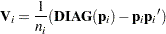
Variance of Probability Estimates |
|||
|
|
|
|
all populations |
|
|
|
Response Functions |
|||
|
|
|
|
all populations |
|
|
|
Derivative of Function with Respect to Probability Estimates |
|||
|
|
|
|
all populations |
|
|
|
Variance of Functions |
|||
|
|
|
|
all populations |
|
|
|
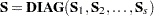
Inverse Variance of Functions |
|||
|
|
|
|
all populations |
|
|
|
 th response


Derivative Table for Compound Functions: Y=F(G(p))
In the following table, let  be a vector of functions of
  , and let
  denote
  , which is the first derivative matrix of
  with respect to :
Function |
|
Derivative |
|---|---|---|
Multiply matrix |
|
|
Logarithm |
|
|
Exponential |
|
|
Add constant |
|
|


Default Response Functions: Generalized Logits
In the following table, subscripts  for the population are suppressed. Also denote
  for
for  for each population
  .
.
Formula |
|
|---|---|
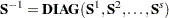
Inverse of Response Functions for a Population |
|
|
|
Form of F and Derivative for a Population |
|
|
|
Covariance Results for a Population |
|
|
|


The following calculations are shown for each population and then for all populations combined:
Source |
Formula |
Dimension |
|
|---|---|---|---|
Design Matrix |
|||
|
|
|
|
all populations |
|
|
|
Crossproduct of Design Matrix |
|||
|
|
|
|
all populations |
|
|
|


In the following table,  is the 100
 th percentile of the standard normal distribution:
Formula |
Dimension |
|
|---|---|---|
Crossproduct of Design Matrix with Function |
||
|
|
|
Weighted Least Squares Estimates |
||
|
|
|
Covariance of Weighted Least Squares Estimates |
||
|
|
|
Wald Confidence Limits for Parameter Estimates |
||
|
|
|
Predicted Response Functions |
||
|
|
|
Covariance of Predicted Response Functions |
||
|
|
|
Residual Chi-Square |
||
RSS |
|
|
Chi-Square for |
||
Q |
|
|


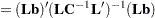
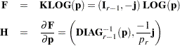
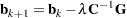
Maximum Likelihood Method
Let  be the Hessian matrix and be the gradient of the log-likelihood function (both functions of
  and the parameters
  ). Let
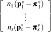
  denote the vector containing the first
  sample proportions from population , and let
  denote the corresponding vector of probability estimates from the current iteration. Starting with the least squares estimates
  of (if you use the ML and WLS options; with the ML option alone, the procedure starts with
  ), the probabilities
  are computed, and
  is calculated iteratively by the Newton-Raphson method until it converges (see the EPSILON= option). The factor
  is a step-halving factor that equals one at the start of each iteration. For any iteration in which the likelihood decreases, PROC CATMOD uses a series of subiterations in which is iteratively divided by two. The subiterations continue until the likelihood is greater than that of the previous iteration. If the likelihood has not reached that point after 10 subiterations, then convergence is assumed, and a warning message is displayed.
Sometimes, infinite parameters are present in the model, either because of the presence of one or more zero frequencies or because of a poorly specified model with collinearity among the estimates. If an estimate is tending toward infinity, then PROC CATMOD flags the parameter as infinite and holds the estimate fixed in subsequent iterations. PROC CATMOD regards a parameter to be infinite when two conditions apply:
The absolute value of its estimate exceeds five divided by the range of the corresponding variable.
The standard error of its estimate is at least three times greater than the estimate itself.
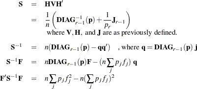
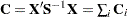
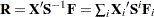
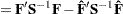
The estimator of the asymptotic covariance matrix of the maximum likelihood predicted probabilities is given by Imrey, Koch, and Stokes (1981, eq. 2.18).
The following equations summarize the method:
 |
where
 |
 |
 |
|||
 |
|
 |
|||
 |
|
 |
Iterative Proportional Fitting
The algorithm used by PROC CATMOD for iterative proportional fitting is described in Bishop, Fienberg, and Holland (1975), Haberman (1972), and Agresti (2002). To illustrate the method, consider the observed three-dimensional table  for the variables X, Y, and Z, and the following hierarchical model:
 |
The following statements request that PROC CATMOD use IPF to fit the preceding model:
model X*Y*Z = _response_ / ml=ipf;
loglin X|Y|Z@2;
Begin with a table of initial cell estimates  . PROC CATMOD produces the initial estimates by setting the
  structural zero cells to 0 and all other cells to
  , where
  is the total weight of the table and
  is the total number of cells in the table. Iteratively adjust the estimates at step
  to the observed marginal tables specified in the model by cycling through the following three-stage process to produce the estimates at step
  :
:
 |
 |
 |
|||
 |
|
 |
|||
 |
|
 |
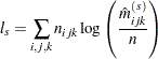
The subscript " " indicates summation over the missing subscript. The log-likelihood
  is estimated at each step by
 |
When the function  is less than
  , the iterations terminate. You can change the comparison value with the EPSILON= option, and you can change the convergence criterion with the CONVCRIT= option. The option CONVCRIT=CELL uses the maximum cell difference
 |
as the criterion while the option CONVCRIT=MARGIN computes the maximum difference of the margins
 |