The ANOVA Procedure

| Randomized Complete Block with One Factor |
This example illustrates the use of PROC ANOVA in analyzing a randomized complete block design. Researchers are interested in whether three treatments have different effects on the yield and worth of a particular crop. They believe that the experimental units are not homogeneous. So, a blocking factor is introduced that allows the experimental units to be homogeneous within each block. The three treatments are then randomly assigned within each block.
The data from this study are input into the SAS data set RCB:
title1 'Randomized Complete Block';
data RCB;
   input Block Treatment $ Yield Worth @@;
   datalines;
1 A 32.6 112   1 B 36.4 130   1 C 29.5 106
2 A 42.7 139   2 B 47.1 143   2 C 32.9 112
3 A 35.3 124   3 B 40.1 134   3 C 33.6 116
;
The variables Yield and Worth are continuous response variables, and the variables Block and Treatment are the classification variables. Because the data for the analysis are balanced, you can use PROC ANOVA to run the analysis.
The statements for the analysis are
proc anova data=RCB;
   class Block Treatment;
   model Yield Worth=Block Treatment;
run;
The Block and Treatment effects appear in the CLASS statement. The MODEL statement requests an analysis for each of the two dependent variables, Yield and Worth.
Figure 24.5 shows the "Class Level Information" table.
| Randomized Complete Block |
| Class Level Information | ||
|---|---|---|
| Class | Levels | Values |
| Block | 3 | 1 2 3 |
| Treatment | 3 | A B C |
| Number of Observations Read | 9 |
|---|---|
| Number of Observations Used | 9 |
The "Class Level Information" table lists the number of levels and their values for all effects specified in the CLASS statement. The number of observations in the data set are also displayed. Use this information to make sure that the data have been read correctly.
The overall ANOVA table for Yield in Figure 24.6 appears first in the output because it is the first response variable listed on the left side in the MODEL statement.
| Randomized Complete Block |
| Source | DF | Sum of Squares | Mean Square | F Value | Pr > F |
|---|---|---|---|---|---|
| Model | 4 | 225.2777778 | 56.3194444 | 8.94 | 0.0283 |
| Error | 4 | 25.1911111 | 6.2977778 | ||
| Corrected Total | 8 | 250.4688889 |
| R-Square | Coeff Var | Root MSE | Yield Mean |
|---|---|---|---|
| 0.899424 | 6.840047 | 2.509537 | 36.68889 |
The overall  statistic is significant
 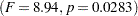 , indicating that the model as a whole accounts for a significant portion of the variation in Yield and that you can proceed to evaluate the tests of effects.
The degrees of freedom (DF) are used to ensure correctness of the data and model. The Corrected Total degrees of freedom are one less than the total number of observations in the data set; in this case,  . The Model degrees of freedom for a randomized complete block are
  , where
  number of block levels and
  number of treatment levels. In this case, this formula leads to
  model degrees of freedom.
Several simple statistics follow the ANOVA table. The R-Square indicates that the model accounts for nearly 90% of the variation in the variable Yield. The coefficient of variation (C.V.) is listed along with the Root MSE and the mean of the dependent variable. The Root MSE is an estimate of the standard deviation of the dependent variable. The C.V. is a unitless measure of variability.
The tests of the effects shown in Figure 24.7 are displayed after the simple statistics.
| Source | DF | Anova SS | Mean Square | F Value | Pr > F |
|---|---|---|---|---|---|
| Block | 2 | 98.1755556 | 49.0877778 | 7.79 | 0.0417 |
| Treatment | 2 | 127.1022222 | 63.5511111 | 10.09 | 0.0274 |
For Yield, both the Block and Treatment effects are significant 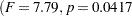 and
and 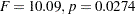 , respectively) at the 95% level. From this you can conclude that blocking is useful for this variable and that some contrast between the treatment means is significantly different from zero.
Figure 24.8 shows the ANOVA table, simple statistics, and tests of effects for the variable Worth.
| Randomized Complete Block |
| Source | DF | Sum of Squares | Mean Square | F Value | Pr > F |
|---|---|---|---|---|---|
| Model | 4 | 1247.333333 | 311.833333 | 8.28 | 0.0323 |
| Error | 4 | 150.666667 | 37.666667 | ||
| Corrected Total | 8 | 1398.000000 |
| R-Square | Coeff Var | Root MSE | Worth Mean |
|---|---|---|---|
| 0.892227 | 4.949450 | 6.137318 | 124.0000 |
| Source | DF | Anova SS | Mean Square | F Value | Pr > F |
|---|---|---|---|---|---|
| Block | 2 | 354.6666667 | 177.3333333 | 4.71 | 0.0889 |
| Treatment | 2 | 892.6666667 | 446.3333333 | 11.85 | 0.0209 |
The overall test is significant 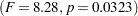 at the 95% level for the variable Worth. The Block effect is not significant at the 0.05 level but is significant at the 0.10 confidence level
 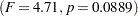 . Generally, the usefulness of blocking should be determined before the analysis. However, since there are two dependent variables of interest, and Block is significant for one of them (Yield), blocking appears to be generally useful. For Worth, as with Yield, the effect of Treatment is significant
 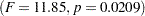 .
.
Issuing the following command produces the Treatment means.
   means Treatment;
run;
Figure 24.9 displays the treatment means and their standard deviations for both dependent variables.
| Randomized Complete Block |
| Level of Treatment |
N | Yield | Worth | ||
|---|---|---|---|---|---|
| Mean | Std Dev | Mean | Std Dev | ||
| A | 3 | 36.8666667 | 5.22908532 | 125.000000 | 13.5277493 |
| B | 3 | 41.2000000 | 5.43415127 | 135.666667 | 6.6583281 |
| C | 3 | 32.0000000 | 2.19317122 | 111.333333 | 5.0332230 |