| The ROBUSTREG Procedure |
| M Estimation |
This example shows how you can use the ROBUSTREG procedure to do M estimation, which is a commonly used method for outlier detection and robust regression when contamination is mainly in the response direction.
data stack;
   input  x1 x2 x3 y exp$ @@;
datalines;
80  27   89  42   e1   80  27   88  37   e2
75  25   90  37   e3   62  24   87  28   e4
62  22   87  18   e5   62  23   87  18   e6
62  24   93  19   e7   62  24   93  20   e8
58  23   87  15   e9   58  18   80  14  e10
58  18   89  14  e11   58  17   88  13  e12
58  18   82  11  e13   58  19   93  12  e14
50  18   89   8  e15   50  18   86   7  e16
50  19   72   8  e17   50  19   79   8  e18
50  20   80   9  e19   56  20   82  15  e20
70  20   91  15  e21
;
The data set stack is the well-known stack-loss data set presented by Brownlee (1965). The data describe the operation of a plant for the oxidation of ammonia to nitric acid and consist of 21 four-dimensional observations. The explanatory variables for the response stack-loss (y) are the rate of operation (x1), the cooling water inlet temperature (x2), and the acid concentration (x3).
The following ROBUSTREG statements analyze the data:
proc robustreg data=stack;
   model y = x1 x2 x3 / diagnostics leverage;
   id    exp;
   test  x3;
run;
By default, the procedure does M estimation with the bisquare weight function, and it uses the median method for estimating the scale parameter. The MODEL statement specifies the covariate effects. The DIAGNOSTICS option requests a table for outlier diagnostics, and the LEVERAGE option adds leverage-point diagnostic results to this table for continuous covariate effects. The ID statement specifies that the variable exp is used to identify each observation (experiment) in this table. If the ID statement is omitted, the observation number is used to identify the observations. The TEST statement requests a test of significance for the covariate effects specified. The results of this analysis are displayed in the following figures.
Figure 75.1 displays the model fitting information and summary statistics for the response variable and the continuous covariates. The columns labeled Q1, Median, and Q3 provide the lower quantile, median, and upper quantile, respectively. The column labeled MAD provides a robust estimate of the univariate scale, which is computed as the standardized median absolute deviation (MAD). See Huber (1981, p. 108) for more details about the standardized MAD. The columns labeled Mean and Standard Deviation provide the usual mean and standard deviation. A large difference between the standard deviation and the MAD for a variable indicates some extreme values for this variable. In the stack-loss data, the stack-loss (response y) has the biggest difference between the standard deviation and the MAD.
| Parameter Estimates | |||||||
|---|---|---|---|---|---|---|---|
| Parameter | DF | Estimate | Standard Error | 95% Confidence Limits | Chi-Square | Pr > ChiSq | |
| Intercept | 1 | -42.2854 | 9.5045 | -60.9138 | -23.6569 | 19.79 | <.0001 |
| x1 | 1 | 0.9276 | 0.1077 | 0.7164 | 1.1387 | 74.11 | <.0001 |
| x2 | 1 | 0.6507 | 0.2940 | 0.0744 | 1.2270 | 4.90 | 0.0269 |
| x3 | 1 | -0.1123 | 0.1249 | -0.3571 | 0.1324 | 0.81 | 0.3683 |
| Scale | 1 | 2.2819 | |||||
Figure 75.2 displays the table of robust parameter estimates, standard errors, and confidence limits. The row labeled Scale provides a point estimate of the scale parameter in the linear regression model, which is obtained by the median method. See the section M Estimation for more information about scale estimation methods. For the stack-loss data, M estimation yields the fitted linear model:
 |
Figure 75.3 displays outlier and leverage-point diagnostics. Standardized robust residuals are computed based on the estimated parameters. Both the Mahalanobis distance and the robust MCD distance are displayed. Outliers and leverage points, identified with asterisks, are defined by the standardized robust residuals and robust MCD distances that exceed the corresponding cutoff values displayed in the diagnostics summary. Observations 4 and 21 are outliers because their standardized robust residuals exceed the cutoff value in absolute value. The procedure detects four observations with high leverage. Leverage points (points with high leverage) with smaller standardized robust residuals than the cutoff value in absolute value are called good leverage points; others are called bad leverage points. Observation 21 is a bad leverage point.
Two particularly useful plots for revealing outliers and leverage points are a scatter plot of the standardized robust residuals against the robust distances (RDPLOT) and a scatter plot of the robust distances against the classical Mahalanobis distances (DDPLOT).
For the stack-loss data, the following statements produce the RDPLOT in Figure 75.4 and the DDPLOT in Figure 75.5. The histogram and the normal quantile-quantile plots (shown in Figure 75.6 and Figure 75.7, respectively) for the standardized robust residuals are also created with the HISTOGRAM and QQPLOT suboptions of the PLOTS= option.
ods graphics on;

proc robustreg data=stack
        plots=(rdplot ddplot histogram qqplot);
   model y = x1 x2 x3;
run;

ods graphics off;
These plots are helpful in identifying outliers in addition to good and bad high leverage points.
These graphical displays are requested by specifying the ODS GRAPHICS statement and the PLOTS= option in the PROC ROBUSTREG statement. For general information about ODS Graphics, see Chapter 21, Statistical Graphics Using ODS. For specific information about the graphics available in the ROBUSTREG procedure, see the section ODS Graphics.
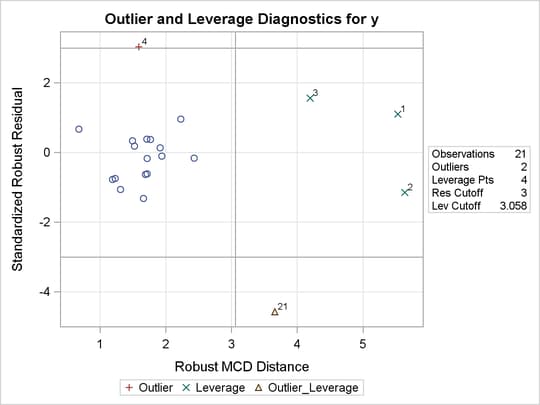
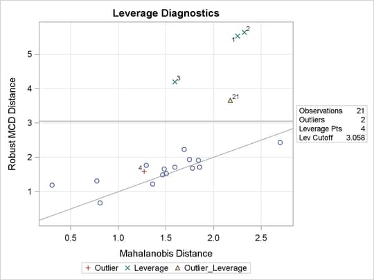
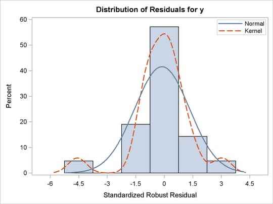
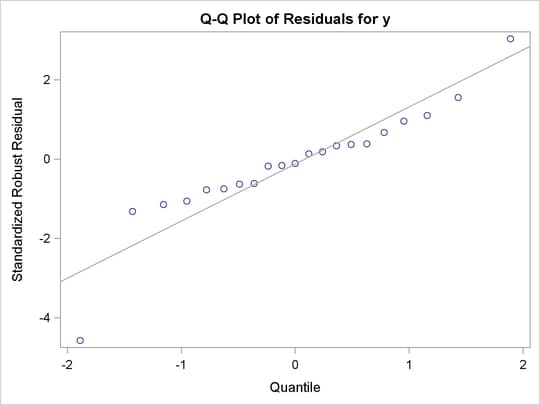
Figure 75.8 displays robust versions of goodness-of-fit statistics for the model. You can use the robust information criteria, AICR and BICR, for model selection and comparison. For both AICR and BICR, the lower the value, the more desirable the model.
Figure 75.9 displays the test results requested by the TEST statement. The ROBUSTREG procedure conducts two robust linear tests, the  test and the
  test. See the section Linear Tests for information about how the procedure computes test statistics and the correction factor lambda. Due to the large
  -values for both tests, you can conclude that the effect x3 is not significant at the
  level.
For the bisquare weight function, the default tuning constant,  , is chosen to yield a
  asymptotic efficiency of the M estimates with the Gaussian distribution. See the section M Estimation for details. The smaller the constant
  , the lower the asymptotic efficiency but the sharper the M estimate as an outlier detector. For the stack-loss data set, you could consider using a sharper outlier detector.
In the following invocation of the ROBUSTREG procedure, a smaller constant,  , is used. This tuning constant corresponds to an efficiency close to
  . See Chen and Yin (2002) for the relationship between the tuning constant and asymptotic efficiency of M estimates.
proc robustreg method=m(wf=bisquare(c=3.5)) data=stack;
   model y = x1 x2 x3 / diagnostics leverage;
   id    exp;
   test  x3;
run;
Figure 75.10 displays the table of robust parameter estimates, standard errors, and confidence limits with the constant .
The refitted linear model is
 |
| Parameter Estimates | |||||||
|---|---|---|---|---|---|---|---|
| Parameter | DF | Estimate | Standard Error | 95% Confidence Limits | Chi-Square | Pr > ChiSq | |
| Intercept | 1 | -37.1076 | 5.4731 | -47.8346 | -26.3805 | 45.97 | <.0001 |
| x1 | 1 | 0.8191 | 0.0620 | 0.6975 | 0.9407 | 174.28 | <.0001 |
| x2 | 1 | 0.5173 | 0.1693 | 0.1855 | 0.8492 | 9.33 | 0.0022 |
| x3 | 1 | -0.0728 | 0.0719 | -0.2138 | 0.0681 | 1.03 | 0.3111 |
| Scale | 1 | 1.4265 | |||||
Figure 75.11 displays outlier and leverage-point diagnostics with the constant . Besides observations 4 and 21, observations 1 and 3 are also detected as outliers.
Copyright © SAS Institute, Inc. All Rights Reserved.