| The PROBIT Procedure |
Example 72.4 An Epidemiology Study
The data in this example, which are from an epidemiology study, consist of five variables: the number, r, of individuals surviving after an epidemic, out of n treated, for combinations of medicine dosage (dose), treatment (treat = A, B), and sex (sex = 0(Female), 1(Male)).
To see whether the two treatments have different effects on male and female individual survival rates, the interaction term between the two variables treat and sex is included in the model.
The following invocation of PROC PROBIT fits the binary probit model to the grouped data:
data epidemic;
   input treat$ dose n r sex @@;
   label dose = Dose;
   datalines;
A  2.17 142 142  0   A   .57 132  47  1
A  1.68 128 105  1   A  1.08 126 100  0
A  1.79 125 118  0   B  1.66 117 115  1
B  1.49 127 114  0   B  1.17  51  44  1
B  2.00 127 126  0   B   .80 129 100  1
;

data xval;
   input treat $ dose sex ;
   datalines;
B  2.  1
;
ods graphics on;

proc probit optc lackfit covout data=epidemic
            outest = out1 xdata = xval
            Plots=(predpplot ippplot lpredplot);
   class treat sex;
   model r/n = dose treat sex sex*treat/corrb covb inversecl;
   output out = out2 p =p;
run;

ods graphics off;
The results of this analysis are shown in the outputs that follow.
Beginning with SAS 8.2, the PROBIT procedure does not support multiple MODEL statements. Only the last one is used if there is more than one MODEL statement in an invocation of the PROBIT procedure.
Output 72.4.1 displays the table of level information for all classification variables in the CLASS statement.
Output 72.4.2 displays the table of parameter information for the effects in the MODEL statement. The name of a parameter is generated by combining the variable names and level names in the effect. The maximum length of a parameter name is 32. The names of the effects are specified in the MODEL statement. The length of names of effects can be specified by the NAMELEN= option in the PROC PROBIT statement, with the default length 20.
Output 72.4.3 displays background information about the model fit. Included are the name of the input data set, the response variables used, and the number of observations, events, and trials. The table also includes the status of the convergence of the model fitting algorithm and the final value of the log-likelihood function.
Output 72.4.4 displays the table of goodness-of-fit tests requested with the LACKFIT option in the PROC PROBIT statement. Two goodness-of-fit statistics, the Pearson’s chi-square statistic and the likelihood ratio chi-square statistic, are computed. The grouping method for computing these statistics can be specified by the AGGREGATE= option. The details can be found in the AGGREGATE= option, and an example can be found in the second part of this example. By default, the PROBIT procedure uses the covariates in the MODEL statement to do grouping. Observations with the same values of the covariates in the MODEL statement are grouped into cells and the two statistics are computed according to these cells. The total number of cells and the number of levels for the response variable are reported next in the "Response-Covariate Profile."
In this example, neither the Pearson’s chi-square nor the log-likelihood ratio chi-square tests are significant at the 0.1 level, which is the default test level used by the PROBIT procedure. That means that the model, which includes the interaction of treat and sex, is suitable for this epidemiology data set. (Further investigation shows that models without the interaction of treat and sex are not acceptable by either test.)
Output 72.4.5 displays the Type III test results for all effects specified in the MODEL statement, which include the degrees of freedom for the effect, the Wald Chi-Square test statistic, and the  -value.
Output 72.4.6 displays the table of parameter estimates for the model. The PROBIT procedure displays information for all the parameters of an effect. Degenerate parameters are indicated by 0 degree of freedom. Confidence intervals are computed for all parameters with nonzero degrees of freedom, including the natural threshold C if the OPTC option is specified in the PROC PROBIT statement. The confidence level can be specified by the ALPHA= option in the MODEL statement. The default confidence level is  .
.
| Analysis of Maximum Likelihood Parameter Estimates | |||||||||
|---|---|---|---|---|---|---|---|---|---|
| Parameter | DF | Estimate | Standard Error | 95% Confidence Limits | Chi-Square | Pr > ChiSq | |||
| Intercept | 1 | -0.8871 | 0.3632 | -1.5991 | -0.1752 | 5.96 | 0.0146 | ||
| dose | 1 | 1.6774 | 0.2583 | 1.1711 | 2.1837 | 42.17 | <.0001 | ||
| treat | A | 1 | -1.2537 | 0.2616 | -1.7664 | -0.7410 | 22.97 | <.0001 | |
| treat | B | 0 | 0.0000 | . | . | . | . | . | |
| sex | 0 | 1 | -0.4633 | 0.2289 | -0.9119 | -0.0147 | 4.10 | 0.0429 | |
| sex | 1 | 0 | 0.0000 | . | . | . | . | . | |
| treat*sex | A | 0 | 1 | 1.2899 | 0.3456 | 0.6126 | 1.9672 | 13.93 | 0.0002 |
| treat*sex | A | 1 | 0 | 0.0000 | . | . | . | . | . |
| treat*sex | B | 0 | 0 | 0.0000 | . | . | . | . | . |
| treat*sex | B | 1 | 0 | 0.0000 | . | . | . | . | . |
| _C_ | 1 | 0.2735 | 0.0946 | 0.0881 | 0.4589 | ||||
From Output 72.4.6, you can see the following results:
The variable dose has a significant positive effect on the survival rate.
Individuals under treatment A have a lower survival rate.
Male individuals have a higher survival rate.
Female individuals under treatment A have a higher survival rate.
Output 72.4.7 and Output 72.4.8 display tables of estimated covariance matrix and estimated correlation matrix for estimated parameters with a nonzero degree of freedom, respectively. They are computed by the inverse of the Hessian matrix of the estimated parameters.
| Estimated Covariance Matrix | ||||||
|---|---|---|---|---|---|---|
| Intercept | dose | treatA | sex0 | treatAsex0 | _C_ | |
| Intercept | 0.131944 | -0.087353 | 0.053551 | 0.030285 | -0.067056 | -0.028073 |
| dose | -0.087353 | 0.066723 | -0.047506 | -0.034081 | 0.058620 | 0.018196 |
| treatA | 0.053551 | -0.047506 | 0.068425 | 0.036063 | -0.075323 | -0.017084 |
| sex0 | 0.030285 | -0.034081 | 0.036063 | 0.052383 | -0.063599 | -0.008088 |
| treatAsex0 | -0.067056 | 0.058620 | -0.075323 | -0.063599 | 0.119408 | 0.019134 |
| _C_ | -0.028073 | 0.018196 | -0.017084 | -0.008088 | 0.019134 | 0.008948 |
| Estimated Correlation Matrix | ||||||
|---|---|---|---|---|---|---|
| Intercept | dose | treatA | sex0 | treatAsex0 | _C_ | |
| Intercept | 1.000000 | -0.930998 | 0.563595 | 0.364284 | -0.534227 | -0.817027 |
| dose | -0.930998 | 1.000000 | -0.703083 | -0.576477 | 0.656744 | 0.744699 |
| treatA | 0.563595 | -0.703083 | 1.000000 | 0.602359 | -0.833299 | -0.690420 |
| sex0 | 0.364284 | -0.576477 | 0.602359 | 1.000000 | -0.804154 | -0.373565 |
| treatAsex0 | -0.534227 | 0.656744 | -0.833299 | -0.804154 | 1.000000 | 0.585364 |
| _C_ | -0.817027 | 0.744699 | -0.690420 | -0.373565 | 0.585364 | 1.000000 |
Output 72.4.9 displays the computed values and fiducial limits for the first single continuous variable dose in the MODEL statement, given the probability levels, without the effect of the natural threshold, and when the option INSERSECL in the MODEL statement is specified. If there is no single continuous variable in the MODEL specification but the INVERSECL option is specified, an error is reported.
| Probit Analysis on dose | |||
|---|---|---|---|
| Probability | dose | 95% Fiducial Limits | |
| 0.01 | -0.85801 | -1.81301 | -0.33743 |
| 0.02 | -0.69549 | -1.58167 | -0.21116 |
| 0.03 | -0.59238 | -1.43501 | -0.13093 |
| 0.04 | -0.51482 | -1.32476 | -0.07050 |
| 0.05 | -0.45172 | -1.23513 | -0.02130 |
| 0.06 | -0.39802 | -1.15888 | 0.02063 |
| 0.07 | -0.35093 | -1.09206 | 0.05742 |
| 0.08 | -0.30877 | -1.03226 | 0.09039 |
| 0.09 | -0.27043 | -0.97790 | 0.12040 |
| 0.10 | -0.23513 | -0.92788 | 0.14805 |
| 0.15 | -0.08900 | -0.72107 | 0.26278 |
| 0.20 | 0.02714 | -0.55706 | 0.35434 |
| 0.25 | 0.12678 | -0.41669 | 0.43322 |
| 0.30 | 0.21625 | -0.29095 | 0.50437 |
| 0.35 | 0.29917 | -0.17477 | 0.57064 |
| 0.40 | 0.37785 | -0.06487 | 0.63387 |
| 0.45 | 0.45397 | 0.04104 | 0.69546 |
| 0.50 | 0.52888 | 0.14481 | 0.75654 |
| 0.55 | 0.60380 | 0.24800 | 0.81819 |
| 0.60 | 0.67992 | 0.35213 | 0.88157 |
| 0.65 | 0.75860 | 0.45879 | 0.94803 |
| 0.70 | 0.84151 | 0.56985 | 1.01942 |
| 0.75 | 0.93099 | 0.68770 | 1.09847 |
| 0.80 | 1.03063 | 0.81571 | 1.18970 |
| 0.85 | 1.14677 | 0.95926 | 1.30171 |
| 0.90 | 1.29290 | 1.12867 | 1.45386 |
| 0.91 | 1.32819 | 1.16747 | 1.49273 |
| 0.92 | 1.36654 | 1.20867 | 1.53590 |
| 0.93 | 1.40870 | 1.25284 | 1.58450 |
| 0.94 | 1.45579 | 1.30084 | 1.64012 |
| 0.95 | 1.50949 | 1.35397 | 1.70515 |
| 0.96 | 1.57258 | 1.41443 | 1.78353 |
| 0.97 | 1.65015 | 1.48626 | 1.88238 |
| 0.98 | 1.75326 | 1.57833 | 2.01720 |
| 0.99 | 1.91577 | 1.71776 | 2.23537 |
If the XDATA= option is used to input a data set for the independent variables in the MODEL statement, the PROBIT procedure uses these values for the independent variables other than the single continuous variable. Missing values are not permitted in the XDATA= data set for the independent variables, although the value for the single continuous variable is not used in the computing of the fiducial limits. A suitable valid value should be given. In the data set xval created by the SAS statements on , dose = 2.
See the section XDATA= SAS-data-set for the default values for those effects other than the single continuous variable, for which the fiducial limits are computed.
In this example, there are two classification variables, treat and sex. Fiducial limits for the dose variable are computed for the highest level of the classification variables, treat = B and sex = 1, which is the default specification. Since these are the default values, you would get the same values and fiducial limits if you did not specify the XDATA= option in this example. The confidence level for the fiducial limits can be specified by the ALPHA= option in the MODEL statement. The default level is .
If a LOG10 or LOG option is used in the PROC PROBIT statement, the values and the fiducial limits are computed for both the single continuous variable and its logarithm.
Output 72.4.10 displays the OUTEST= data set. All parameters for an effect are included.
| Obs | _MODEL_ | _NAME_ | _TYPE_ | _DIST_ | _STATUS_ | _LNLIKE_ | r | Intercept | dose | treatA | treatB | sex0 | sex1 | treatAsex0 | treatAsex1 | treatBsex0 | treatBsex1 | _C_ |
|---|---|---|---|---|---|---|---|---|---|---|---|---|---|---|---|---|---|---|
| 1 | r | PARMS | Normal | 0 Converged | -387.247 | -1.00000 | -0.88714 | 1.67739 | -1.25367 | 0 | -0.46329 | 0 | 1.28991 | 0 | 0 | 0 | 0.27347 | |
| 2 | Intercept | COV | Normal | 0 Converged | -387.247 | -0.88714 | 0.13194 | -0.08735 | 0.05355 | 0 | 0.03029 | 0 | -0.06706 | 0 | 0 | 0 | -0.02807 | |
| 3 | dose | COV | Normal | 0 Converged | -387.247 | 1.67739 | -0.08735 | 0.06672 | -0.04751 | 0 | -0.03408 | 0 | 0.05862 | 0 | 0 | 0 | 0.01820 | |
| 4 | treatA | COV | Normal | 0 Converged | -387.247 | -1.25367 | 0.05355 | -0.04751 | 0.06843 | 0 | 0.03606 | 0 | -0.07532 | 0 | 0 | 0 | -0.01708 | |
| 5 | treatB | COV | Normal | 0 Converged | -387.247 | 0.00000 | 0.00000 | 0.00000 | 0.00000 | 0 | 0.00000 | 0 | 0.00000 | 0 | 0 | 0 | 0.00000 | |
| 6 | sex0 | COV | Normal | 0 Converged | -387.247 | -0.46329 | 0.03029 | -0.03408 | 0.03606 | 0 | 0.05238 | 0 | -0.06360 | 0 | 0 | 0 | -0.00809 | |
| 7 | sex1 | COV | Normal | 0 Converged | -387.247 | 0.00000 | 0.00000 | 0.00000 | 0.00000 | 0 | 0.00000 | 0 | 0.00000 | 0 | 0 | 0 | 0.00000 | |
| 8 | treatAsex0 | COV | Normal | 0 Converged | -387.247 | 1.28991 | -0.06706 | 0.05862 | -0.07532 | 0 | -0.06360 | 0 | 0.11941 | 0 | 0 | 0 | 0.01913 | |
| 9 | treatAsex1 | COV | Normal | 0 Converged | -387.247 | 0.00000 | 0.00000 | 0.00000 | 0.00000 | 0 | 0.00000 | 0 | 0.00000 | 0 | 0 | 0 | 0.00000 | |
| 10 | treatBsex0 | COV | Normal | 0 Converged | -387.247 | 0.00000 | 0.00000 | 0.00000 | 0.00000 | 0 | 0.00000 | 0 | 0.00000 | 0 | 0 | 0 | 0.00000 | |
| 11 | treatBsex1 | COV | Normal | 0 Converged | -387.247 | 0.00000 | 0.00000 | 0.00000 | 0.00000 | 0 | 0.00000 | 0 | 0.00000 | 0 | 0 | 0 | 0.00000 | |
| 12 | _C_ | COV | Normal | 0 Converged | -387.247 | 0.27347 | -0.02807 | 0.01820 | -0.01708 | 0 | -0.00809 | 0 | 0.01913 | 0 | 0 | 0 | 0.00895 |
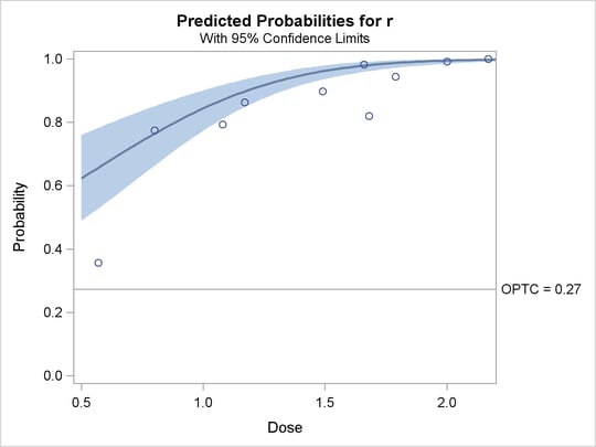
The plots in the following three outputs, Output 72.4.11, Output 72.4.12, and Output 72.4.13, are generated by the PLOTS= option. The first plot, specified with the PREDPPLOT option, is the plot of the predicted probability against the first single continuous variable dose in the MODEL statement. You can specify values of other independent variables in the MODEL statement by using an XDATA= data set or by using the default values.
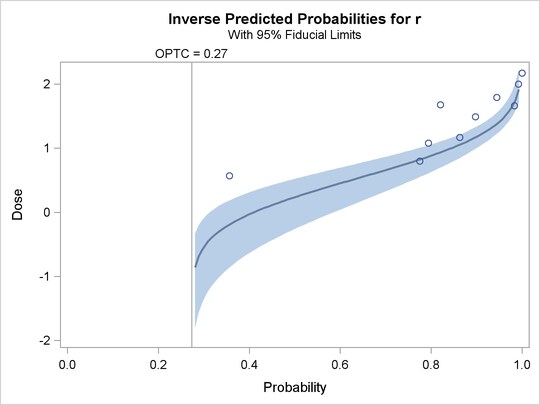
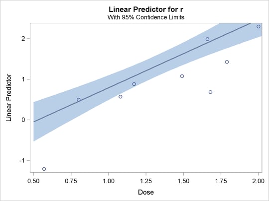
The second plot, specified with the IPPPLOT option, is the inverse of the predicted probability plot with the fiducial limits. It should be pointed out that the fiducial limits are not just the inverse of the confidence limits in the predicted probability plot; see the section Inverse Confidence Limits for the computation of these limits. The third plot, specified with the LPREDPLOT option, is the plot of the linear predictor  against the first single continuous variable with the Wald confidence intervals.
When you combine the INEST= data set and the MAXIT= option in the MODEL statement, the PROBIT procedure can do prediction, if the parameterizations for the models used for the training data and the validation data are exactly the same. The following SAS statements show an example:
data validate;
   input treat $ dose  sex  n r group @@;
   datalines;
B  2.0  0  44 43  1   B  2.0  1  54 52  2
B  1.5  1  36 32  3   B  1.5  0  45 40  4
A  2.0  0  66 64  5   A  2.0  1  89 89  6
A  1.5  1  45 39  7   A  1.5  0  66 60  8
B  2.0  0  44 44  1   B  2.0  1  54 54  2
B  1.5  1  36 30  3   B  1.5  0  45 41  4
A  2.0  0  66 65  5   A  2.0  1  89 88  6
A  1.5  1  45 38  7   A  1.5  0  66 59  8
;
proc probit optc data=validate inest=out1;
   class treat sex;
   model r/n = dose treat sex sex*treat  / maxit = 0 ;
   output out = out3 p =p;
run ;
proc probit optc lackfit data=validate inest=out1;
   class treat sex;
   model r/n = dose treat sex sex*treat / aggregate = group ;
   output out = out4 p =p;
run ;
After the first invocation of PROC PROBIT, you have the estimated parameters and their covariance matrix in the data set OUTEST = Out1, and the fitted probabilities for the training data set epidemic in the data set OUTPUT = Out2. See Output 72.4.10 for the data set Out1 and Output 72.4.14 for the data set Out2.
The validation data are collected in data set validate. The second invocation of PROC PROBIT simply passes the estimated parameters from the training data set epidemic to the validation data set validate for prediction. The predicted probabilities are stored in the data set OUTPUT = Out3 (see Output 72.4.15). The third invocation of PROC PROBIT passes the estimated parameters as initial values for a new fit of the validation data set with the same model. Predicted probabilities are stored in the data set OUTPUT = Out4 (see Output 72.4.16). Goodness-of-fit tests are computed based on the cells grouped by the AGGREGATE= group variable. Results are shown in Output 72.4.17.
| Obs | treat | dose | sex | n | r | group | p |
|---|---|---|---|---|---|---|---|
| 1 | B | 2.0 | 0 | 44 | 43 | 1 | 0.98364 |
| 2 | B | 2.0 | 1 | 54 | 52 | 2 | 0.99506 |
| 3 | B | 1.5 | 1 | 36 | 32 | 3 | 0.96247 |
| 4 | B | 1.5 | 0 | 45 | 40 | 4 | 0.91145 |
| 5 | A | 2.0 | 0 | 66 | 64 | 5 | 0.98500 |
| 6 | A | 2.0 | 1 | 89 | 89 | 6 | 0.91835 |
| 7 | A | 1.5 | 1 | 45 | 39 | 7 | 0.74300 |
| 8 | A | 1.5 | 0 | 66 | 60 | 8 | 0.91666 |
| 9 | B | 2.0 | 0 | 44 | 44 | 1 | 0.98364 |
| 10 | B | 2.0 | 1 | 54 | 54 | 2 | 0.99506 |
| 11 | B | 1.5 | 1 | 36 | 30 | 3 | 0.96247 |
| 12 | B | 1.5 | 0 | 45 | 41 | 4 | 0.91145 |
| 13 | A | 2.0 | 0 | 66 | 65 | 5 | 0.98500 |
| 14 | A | 2.0 | 1 | 89 | 88 | 6 | 0.91835 |
| 15 | A | 1.5 | 1 | 45 | 38 | 7 | 0.74300 |
| 16 | A | 1.5 | 0 | 66 | 59 | 8 | 0.91666 |
| Obs | treat | dose | sex | n | r | group | p |
|---|---|---|---|---|---|---|---|
| 1 | B | 2.0 | 0 | 44 | 43 | 1 | 0.98954 |
| 2 | B | 2.0 | 1 | 54 | 52 | 2 | 0.98262 |
| 3 | B | 1.5 | 1 | 36 | 32 | 3 | 0.86187 |
| 4 | B | 1.5 | 0 | 45 | 40 | 4 | 0.90095 |
| 5 | A | 2.0 | 0 | 66 | 64 | 5 | 0.98768 |
| 6 | A | 2.0 | 1 | 89 | 89 | 6 | 0.98614 |
| 7 | A | 1.5 | 1 | 45 | 39 | 7 | 0.88075 |
| 8 | A | 1.5 | 0 | 66 | 60 | 8 | 0.88964 |
| 9 | B | 2.0 | 0 | 44 | 44 | 1 | 0.98954 |
| 10 | B | 2.0 | 1 | 54 | 54 | 2 | 0.98262 |
| 11 | B | 1.5 | 1 | 36 | 30 | 3 | 0.86187 |
| 12 | B | 1.5 | 0 | 45 | 41 | 4 | 0.90095 |
| 13 | A | 2.0 | 0 | 66 | 65 | 5 | 0.98768 |
| 14 | A | 2.0 | 1 | 89 | 88 | 6 | 0.98614 |
| 15 | A | 1.5 | 1 | 45 | 38 | 7 | 0.88075 |
| 16 | A | 1.5 | 0 | 66 | 59 | 8 | 0.88964 |
Copyright © SAS Institute, Inc. All Rights Reserved.