| The PROBIT Procedure |
| Inverse Confidence Limits |
In bioassay problems, estimates of the values of the independent variables that yield a desired response are often needed. For instance, the value yielding a 50% response rate (called the ED50 or LD50) is often used. The INVERSECL option requests that confidence limits be computed for the value of the independent variable that yields a specified response. These limits are computed only for the first continuous variable effect in the model. The other variables are set either at their mean values if they are continuous or at the reference (last) level if they are discrete variables. For a discussion of inverse confidence limits, see Hubert, Bohidar, and Peace (1988).
For the PROBIT procedure, the response variable is a probability. An estimate of the first continuous variable value needed to achieve a response of  is given by
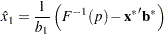 |
where  is the cumulative distribution function used to model the probability,
  is the vector of independent variables excluding the first one, which can be specified by the XDATA= option described in the section XDATA= SAS-data-set,
  is the vector of parameter estimates excluding the first one, and
  is the estimated regression coefficient for the independent variable of interest. This estimate assumes that there is no natural response rate (
 ). When
  is nonzero, the quantiles and confidence limits for the independent variable correspond to the adjusted probability
  , rather than to . As a result, an estimate of the value yielding response rate is associated with the
  quantile. For example, if
  then an estimate of the LD50 is found corresponding to the 0.44 quantile. This value can be thought of as yielding 50% of the variable’s effect, but a 44% response rate. For both binary and ordinal models, the INVERSECL option provides estimates of the value of
  , which yields
  , for various values of .
This estimator is given as a ratio of random variables, such as  . Confidence limits for this ratio can be computed by using Fieller’s theorem. A brief description of this theorem follows. See Finney (1971) for a more complete description of Fieller’s theorem.
If the random variables  and
and  are thought to be distributed as jointly normal, then for any fixed value
  the following probability statement holds if
  is an
is an  quantile from the standard normal distribution and
  is the variance-covariance matrix of a and :
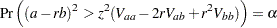 |
Usually the inequality can be solved for to yield a confidence interval. The PROBIT procedure uses a value of 1.96 for , corresponding to an  value of 0.05, unless the goodness-of-fit -value is less than the specified value of the HPROB= option. When this happens, the covariance matrix is scaled by the heterogeneity factor, and a
  distribution quantile is used for .
It is possible for the roots of the equation for to be imaginary or for the confidence interval to be all points outside of an interval. In these cases, the limits are set to missing by the PROBIT procedure.
Although the normal and logistic distribution give comparable fitted values of if the empirically observed proportions are not too extreme, they can give appreciably different values when extrapolated into the tails. Correspondingly, the estimates of the confidence limits and dose values can be different for the two distributions even when they agree quite well in the body of the data. Extrapolation outside of the range of the actual data is often sensitive to model assumptions, and caution is advised if extrapolation is necessary.
It should be pointed out that, when there is a natural threshold , the quantiles and confidence limits for the independent variable correspond to the adjusted probability .
Copyright © SAS Institute, Inc. All Rights Reserved.