Fine-Tuning a Sample Size Axis

Consider the following plot request for a sample size analysis similar to the one in Output 68.8.1 but with only a single scenario, and with unbalanced sample size allocation of 2:1:

proc power plotonly;
   ods output plotcontent=PlotData;
   twosamplemeans test=diff
      groupmeans   = 12 | 18
      stddev       = 7
      groupweights = 2 | 1
      power        = .
      ntotal       = 20;
   plot x=n min=20 max=50 npoints=20;
run;

The MIN=, MAX=, and NPOINTS= options in the PLOT statement request a plot with 20 points between 20 and 50. But the resulting plot (Output 68.8.7) appears to have only 11 points, and they range from 18 to 48.

Output 68.8.7 Plot with Overlapping Points

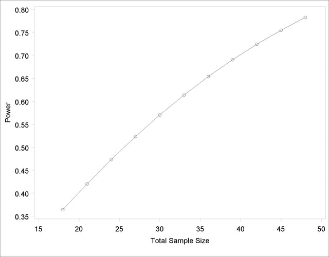
The reason that this plot has fewer points than usual is due to the rounding of sample sizes. If you do not use the NFRACTIONAL option in the analysis statement (here, the TWOSAMPLEMEANS statement), then the set of sample size points determined by the MIN=, MAX=, NPOINTS=, and STEP= options in the PLOT statement can be rounded to satisfy the allocation weights. In this case, they are rounded down to the nearest multiples of 3 (the sum of the weights), and many of the points overlap. To see the overlap, you can print the NominalNTotal (unadjusted) and NTotal (rounded) variables in the PlotContent ODS object (here saved to a data set called PlotData):

proc print data=PlotData;
   var NominalNTotal NTotal;
run;

The output is shown in Output 68.8.8.

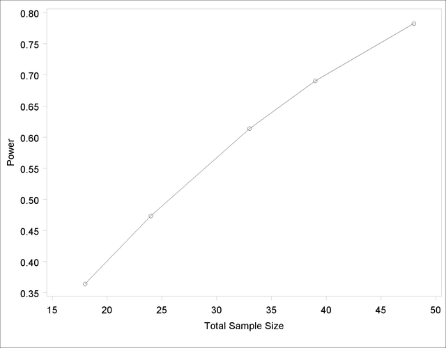
Besides overlapping of sample size points, another peculiarity that might occur without the NFRACTIONAL option is unequal spacing—for example, in the plot in Output 68.8.9, created with the following statements:

proc power plotonly;
   twosamplemeans test=diff
      groupmeans   = 12 | 18
      stddev       = 7
      groupweights = 2 | 1
      power        = .
      ntotal       = 20;
   plot x=n min=20 max=50 npoints=5;
run;

Output 68.8.9 Plot with Unequally Spaced Points

If you want to guarantee evenly spaced, nonoverlapping sample size points in your plots, you can either (1) use the NFRACTIONAL option in the analysis statement preceding the PLOT statement or (2) use the STEP= option and provide values for the MIN=, MAX=, and STEP= options in the PLOT statement that are multiples of the sum of the allocation weights. Note that this sum is simply 1 for one-sample and paired designs and 2 for balanced two-sample designs. So any integer step value works well for one-sample and paired designs, and any even step value works well for balanced two-sample designs. Both of these strategies will avoid rounding adjustments.

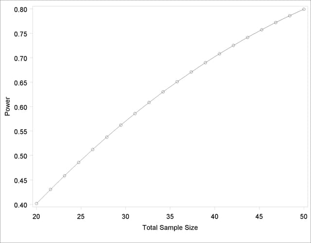
The following statements implement the first strategy to create the plot in Output 68.8.10, by using the NFRACTIONAL option in the TWOSAMPLEMEANS statement:

proc power plotonly;
   twosamplemeans test=diff
      nfractional
      groupmeans   = 12 | 18
      stddev       = 7
      groupweights = 2 | 1
      power        = .
      ntotal       = 20;
   plot x=n min=20 max=50 npoints=20;
run;

Output 68.8.10 Plot with Fractional Sample Sizes

To implement the second strategy, use multiples of 3 for the STEP=, MIN=, and MAX= options in the PLOT statement (because the sum of the allocation weights is ). The following statements use STEP=3, MIN=18, and MAX=48 to create a plot that looks identical to the plot in Output 68.8.7 but suffers no overlapping of points:

proc power plotonly;
   twosamplemeans test=diff
      groupmeans   = 12 | 18
      stddev       = 7
      groupweights = 2 | 1
      power        = .
      ntotal       = 20;
   plot x=n min=18 max=48 step=3;
run;