| The MIXED Procedure |
Example 56.8 Influence Analysis for Repeated Measures Data
This example revisits the repeated measures data of Pothoff and Roy (1964) that were analyzed in Example 56.2. Recall that the data consist of growth measurements at ages 8, 10, 12, and 14 for 11 girls and 16 boys. The model being fit contains fixed effects for Gender and Age and their interaction.
The earlier analysis of these data indicated some unusual observations in this data set. Because of the clustered data structure, it is of interest to study the influence of clusters (children) on the analysis rather than the influence of individual observations. A cluster comprises the repeated measurements for each child.
The repeated measures are first modeled with an unstructured within-child variance-covariance matrix. A residual variance is not profiled in this model. A noniterative influence analysis will update the fixed effects only. The following statements request this noniterative maximum likelihood analysis and produce Output 56.8.1:
proc mixed data=pr method=ml;
  class person gender;
  model y = gender age gender*age /
                   influence(effect=person);
  repeated / type=un subject=person;
  ods select influence;
run;
| Influence Diagnostics for Levels of Person |
|||
|---|---|---|---|
| Person | Number of Observations in Level |
PRESS Statistic | Cook's D |
| 1 | 4 | 10.1716 | 0.01539 |
| 2 | 4 | 3.8187 | 0.03988 |
| 3 | 4 | 10.8448 | 0.02891 |
| 4 | 4 | 24.0339 | 0.04515 |
| 5 | 4 | 1.6900 | 0.01613 |
| 6 | 4 | 11.8592 | 0.01634 |
| 7 | 4 | 1.1887 | 0.00521 |
| 8 | 4 | 4.6717 | 0.02742 |
| 9 | 4 | 13.4244 | 0.03949 |
| 10 | 4 | 85.1195 | 0.13848 |
| 11 | 4 | 67.9397 | 0.09728 |
| 12 | 4 | 40.6467 | 0.04438 |
| 13 | 4 | 13.0304 | 0.00924 |
| 14 | 4 | 6.1712 | 0.00411 |
| 15 | 4 | 24.5702 | 0.12727 |
| 16 | 4 | 20.5266 | 0.01026 |
| 17 | 4 | 9.9917 | 0.01526 |
| 18 | 4 | 7.9355 | 0.01070 |
| 19 | 4 | 15.5955 | 0.01982 |
| 20 | 4 | 42.6845 | 0.01973 |
| 21 | 4 | 95.3282 | 0.10075 |
| 22 | 4 | 13.9649 | 0.03778 |
| 23 | 4 | 4.9656 | 0.01245 |
| 24 | 4 | 37.2494 | 0.15094 |
| 25 | 4 | 4.3756 | 0.03375 |
| 26 | 4 | 8.1448 | 0.03470 |
| 27 | 4 | 20.2913 | 0.02523 |
Each observation in the "Influence Diagnostics for Levels of Person" table in Output 56.8.1 represents the removal of four observations. The subjects 10, 15, and 24 have the greatest impact on the fixed effects (Cook’s  ), and subject 10 and 21 have large PRESS statistics. The 21st child has a large PRESS statistic, and its statistic is not that extreme. This is an indication that the model fits rather poorly for this child, whether it is part of the data or not.
The previous analysis does not take into account the effect on the covariance parameters when a subject is removed from the analysis. If you also update the covariance parameters, the impact of observations on these can amplify or allay their effect on the fixed effects. To assess the overall influence of subjects on the analysis and to compute separate statistics for the fixed effects and covariance parameters, an iterative analysis is obtained by adding the INFLUENCE suboption ITER=, as follows:
ods graphics on;

proc mixed data=pr method=ml;
  class person gender;
  model y = gender age gender*age /
                   influence(effect=person iter=5);
  repeated / type=un subject=person;
run;
The number of additional iterations following removal of the observations for a particular subject is limited to five. Graphical displays of influence diagnostics are requested by specifying the ODS GRAPHICS statement. For general information about ODS Graphics, see Chapter 21, Statistical Graphics Using ODS. For specific information about the graphics available in the MIXED procedure, see the section ODS Graphics.
The MIXED procedure produces a plot of the restricted likelihood distance (Output 56.8.2) and a panel of diagnostics for fixed effects and covariance parameters (Output 56.8.3).
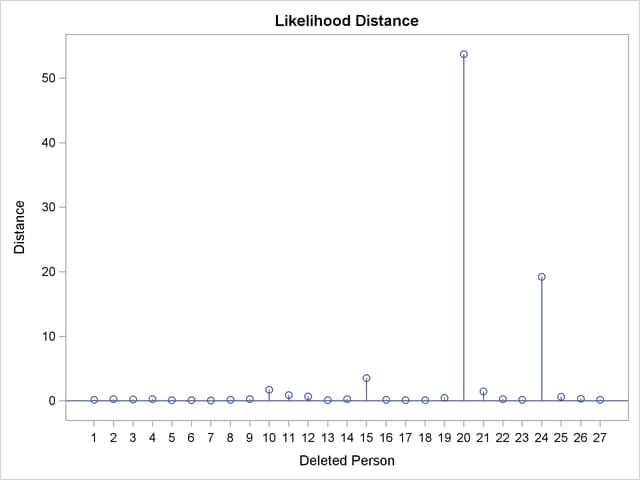
As judged by the restricted likelihood distance, subjects 20 and 24 clearly have the most influence on the overall analysis (Output 56.8.2).
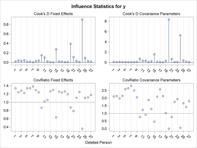
Output 56.8.3 displays Cook’s and CovRatio statistics for the fixed effects and covariance parameters. Clearly, subject 20 has a dramatic effect on the estimates of variances and covariances. This subject also affects the precision of the covariance parameter estimates more than any other subject in Output 56.8.3 (CovRatio near 0).
The child who exerts the greatest influence on the fixed effects is subject 24. Maybe surprisingly, this subject affects the variance-covariance matrix of the fixed effects more than subject 20 (small CovRatio in Output 56.8.3).
The final model investigated for these data is a random coefficient model as in Stram and Lee (1994) with random effects for the intercept and age effect. The following statements examine the estimates for fixed effects and the entries of the unstructured  variance matrix of the random coefficients graphically:
proc mixed data=pr method=ml
           plots(only)=InfluenceEstPlot;
   class person gender;
   model y = gender age gender*age /
                    influence(iter=5 effect=person est);
   random intercept age / type=un subject=person;
run;
The PLOTS(ONLY)=INFLUENCEESTPLOT option restricts the graphical output from this PROC MIXED run to only the panels of deletion estimates (Output 56.8.4 and Output 56.8.5).
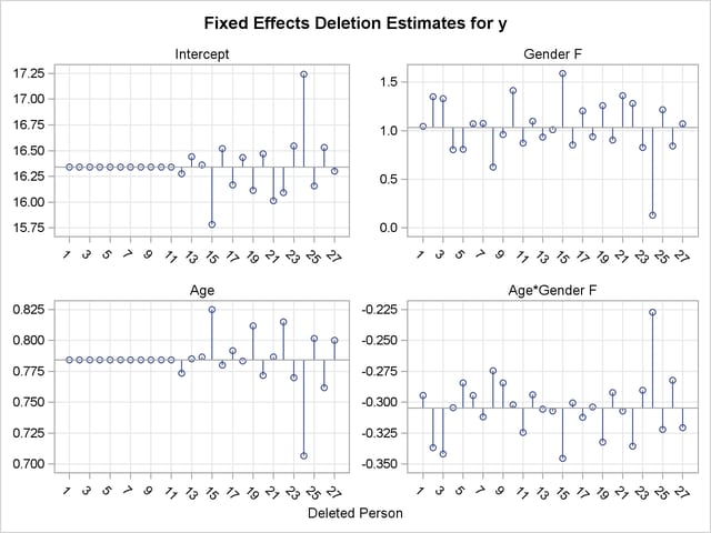
In Output 56.8.4 the graphs on the left side of the panel represent the intercept and slope estimate for boys; the graphs on the right side represent the difference in intercept and slope between boys and girls. Removing any one of the first eleven children, who are girls, does not alter the intercept or slope in the group of boys. The difference in these parameters between boys and girls is altered by the removal of any child. Subject 24 changes the fixed effects considerably, subject 20 much less so.
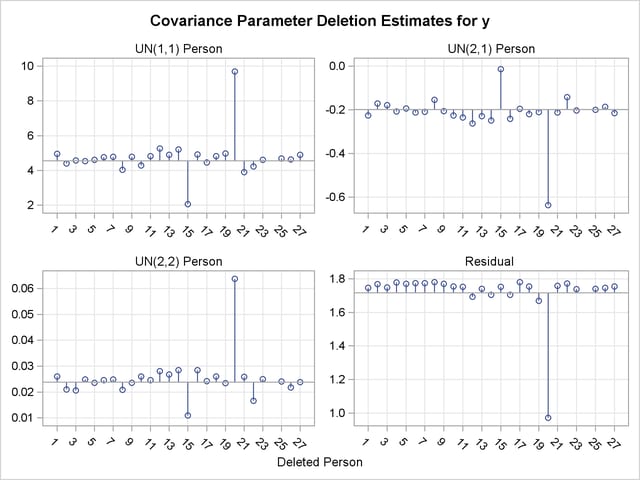
The covariance parameter deletion estimates in Output 56.8.5 show several important features.
The panels do not contain information about subject 24. Estimation of the
 matrix following removal of that child did not yield a positive definite matrix. As a consequence, covariance parameter diagnostics are not produced for this subject.
 Subject 20 has great impact on the four covariance parameters. Removing this child from the analysis increases the variance of the random intercept and random slope and reduces the residual variance by almost 80%. The repeated measurements of this child exhibit an up-and-down behavior.
The variance of the random intercept and slope are reduced when child 15 is removed from the analysis. This child’s growth measurements oscillate about 27.0 from age 10 on.
Examining observed and residual values by levels of classification variables is also a useful tool to diagnose the adequacy of the model and unusual observations. Box plots for effects in the model that consist of only classification variables can be requested with the BOXPLOT option of the PLOTS= option in the PROC MIXED statement. For example, the following statements produce box plots for the SUBJECT= effects in the model:
proc mixed data=pr method=ml
       plot=boxplot(observed marginal conditional subject);
   class person gender;
   model y = gender age gender*age;
   random intercept age / type=un subject=person;
run;
The specific boxplot options request a plot of the observed data (Output 56.8.6), the marginal residuals (Output 56.8.7), and the conditional residuals (Output 56.8.8). Box plots of the observed values show the variation within and between children clearly. The group of girls (subjects 1–11) is distinguishable from the group of boys by somewhat lesser average growth and lesser within-child variation (Output 56.8.6). After adjusting for overall (population-averaged) gender and age effects, the residual within-child variation is reduced but substantial differences in the means remain (Output 56.8.7). If child-specific inferences are desired, a model accounting for only Gender, Age, and Gender*Age effects is not adequate for these data.
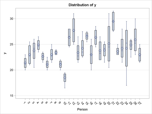
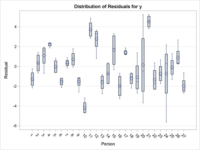
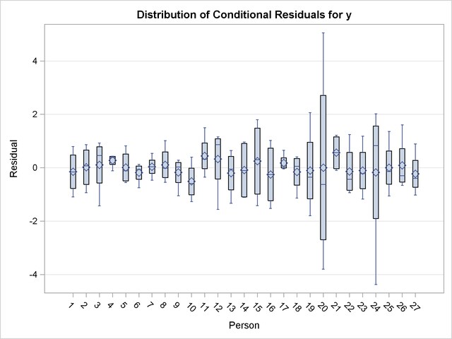
The conditional residuals incorporate the EBLUPs for each child and enable you to examine whether the subject-specific model is adequate (Output 56.8.8). By using each child "as its own control," the residuals are now centered near zero. Subjects 20 and 24 stand out as unusual in all three sets of box plots.
Copyright © SAS Institute, Inc. All Rights Reserved.