| The LOGISTIC Procedure |
Example 51.6 Logistic Regression Diagnostics
In a controlled experiment to study the effect of the rate and volume of air intake on a transient reflex vasoconstriction in the skin of the digits, 39 tests under various combinations of rate and volume of air intake were obtained (Finney; 1947). The endpoint of each test is whether or not vasoconstriction occurred. Pregibon (1981) uses this set of data to illustrate the diagnostic measures he proposes for detecting influential observations and to quantify their effects on various aspects of the maximum likelihood fit.
The vasoconstriction data are saved in the data set vaso:
data vaso;
   length Response $12;
   input Volume Rate Response @@;
   LogVolume=log(Volume);
   LogRate=log(Rate);
   datalines;
3.70  0.825  constrict       3.50  1.09   constrict
1.25  2.50   constrict       0.75  1.50   constrict
0.80  3.20   constrict       0.70  3.50   constrict
0.60  0.75   no_constrict    1.10  1.70   no_constrict
0.90  0.75   no_constrict    0.90  0.45   no_constrict
0.80  0.57   no_constrict    0.55  2.75   no_constrict
0.60  3.00   no_constrict    1.40  2.33   constrict
0.75  3.75   constrict       2.30  1.64   constrict
3.20  1.60   constrict       0.85  1.415  constrict
1.70  1.06   no_constrict    1.80  1.80   constrict
0.40  2.00   no_constrict    0.95  1.36   no_constrict
1.35  1.35   no_constrict    1.50  1.36   no_constrict
1.60  1.78   constrict       0.60  1.50   no_constrict
1.80  1.50   constrict       0.95  1.90   no_constrict
1.90  0.95   constrict       1.60  0.40   no_constrict
2.70  0.75   constrict       2.35  0.03   no_constrict
1.10  1.83   no_constrict    1.10  2.20   constrict
1.20  2.00   constrict       0.80  3.33   constrict
0.95  1.90   no_constrict    0.75  1.90   no_constrict
1.30  1.625  constrict
;
In the data set vaso, the variable Response represents the outcome of a test. The variable LogVolume represents the log of the volume of air intake, and the variable LogRate represents the log of the rate of air intake.
The following statements invoke PROC LOGISTIC to fit a logistic regression model to the vasoconstriction data, where Response is the response variable, and LogRate and LogVolume are the explanatory variables. The ODS GRAPHICS ON statement is specified to display the regression diagnostics, and the INFLUENCE option is specified to display a table of the regression diagnostics.
ods graphics on;
title 'Occurrence of Vasoconstriction';
proc logistic data=vaso;
   model Response=LogRate LogVolume/influence iplots;
run;
ods graphics off;
Results of the model fit are shown in Output 51.6.1. Both LogRate and LogVolume are statistically significant to the occurrence of vasoconstriction ( and
and  , respectively). Their positive parameter estimates indicate that a higher inspiration rate or a larger volume of air intake is likely to increase the probability of vasoconstriction.
| Occurrence of Vasoconstriction |
| Model Information | |
|---|---|
| Data Set | WORK.VASO |
| Response Variable | Response |
| Number of Response Levels | 2 |
| Model | binary logit |
| Optimization Technique | Fisher's scoring |
| Response Profile | ||
|---|---|---|
| Ordered Value |
Response | Total Frequency |
| 1 | constrict | 20 |
| 2 | no_constrict | 19 |
| Model Fit Statistics | ||
|---|---|---|
| Criterion | Intercept Only |
Intercept and Covariates |
| AIC | 56.040 | 35.227 |
| SC | 57.703 | 40.218 |
| -2 Log L | 54.040 | 29.227 |
| Testing Global Null Hypothesis: BETA=0 | |||
|---|---|---|---|
| Test | Chi-Square | DF | Pr > ChiSq |
| Likelihood Ratio | 24.8125 | 2 | <.0001 |
| Score | 16.6324 | 2 | 0.0002 |
| Wald | 7.8876 | 2 | 0.0194 |
| Analysis of Maximum Likelihood Estimates | |||||
|---|---|---|---|---|---|
| Parameter | DF | Estimate | Standard Error |
Wald Chi-Square |
Pr > ChiSq |
| Intercept | 1 | -2.8754 | 1.3208 | 4.7395 | 0.0295 |
| LogRate | 1 | 4.5617 | 1.8380 | 6.1597 | 0.0131 |
| LogVolume | 1 | 5.1793 | 1.8648 | 7.7136 | 0.0055 |
The INFLUENCE option displays the values of the explanatory variables (LogRate and LogVolume) for each observation, a column for each diagnostic produced, and the case number that represents the sequence number of the observation (Output 51.6.2). Also produced (but suppressed by the ODS GRAPHICS statement) is a line-printer plot where the vertical axis represents the case number and the horizontal axis represents the value of the diagnostic statistic.
| Regression Diagnostics | ||||||||||||
|---|---|---|---|---|---|---|---|---|---|---|---|---|
| Case Number |
Covariates | Pearson Residual | Deviance Residual | Hat Matrix Diagonal | Intercept DfBeta | LogRate DfBeta | LogVolume DfBeta | Confidence Interval Displacement C |
Confidence Interval Displacement CBar |
Delta Deviance | Delta Chi-Square | |
| LogRate | LogVolume | |||||||||||
| 1 | -0.1924 | 1.3083 | 0.2205 | 0.3082 | 0.0927 | -0.0165 | 0.0193 | 0.0556 | 0.00548 | 0.00497 | 0.1000 | 0.0536 |
| 2 | 0.0862 | 1.2528 | 0.1349 | 0.1899 | 0.0429 | -0.0134 | 0.0151 | 0.0261 | 0.000853 | 0.000816 | 0.0369 | 0.0190 |
| 3 | 0.9163 | 0.2231 | 0.2923 | 0.4049 | 0.0612 | -0.0492 | 0.0660 | 0.0589 | 0.00593 | 0.00557 | 0.1695 | 0.0910 |
| 4 | 0.4055 | -0.2877 | 3.5181 | 2.2775 | 0.0867 | 1.0734 | -0.9302 | -1.0180 | 1.2873 | 1.1756 | 6.3626 | 13.5523 |
| 5 | 1.1632 | -0.2231 | 0.5287 | 0.7021 | 0.1158 | -0.0832 | 0.1411 | 0.0583 | 0.0414 | 0.0366 | 0.5296 | 0.3161 |
| 6 | 1.2528 | -0.3567 | 0.6090 | 0.7943 | 0.1524 | -0.0922 | 0.1710 | 0.0381 | 0.0787 | 0.0667 | 0.6976 | 0.4376 |
| 7 | -0.2877 | -0.5108 | -0.0328 | -0.0464 | 0.00761 | -0.00280 | 0.00274 | 0.00265 | 8.321E-6 | 8.258E-6 | 0.00216 | 0.00109 |
| 8 | 0.5306 | 0.0953 | -1.0196 | -1.1939 | 0.0559 | -0.1444 | 0.0613 | 0.0570 | 0.0652 | 0.0616 | 1.4870 | 1.1011 |
| 9 | -0.2877 | -0.1054 | -0.0938 | -0.1323 | 0.0342 | -0.0178 | 0.0173 | 0.0153 | 0.000322 | 0.000311 | 0.0178 | 0.00911 |
| 10 | -0.7985 | -0.1054 | -0.0293 | -0.0414 | 0.00721 | -0.00245 | 0.00246 | 0.00211 | 6.256E-6 | 6.211E-6 | 0.00172 | 0.000862 |
| 11 | -0.5621 | -0.2231 | -0.0370 | -0.0523 | 0.00969 | -0.00361 | 0.00358 | 0.00319 | 0.000014 | 0.000013 | 0.00274 | 0.00138 |
| 12 | 1.0116 | -0.5978 | -0.5073 | -0.6768 | 0.1481 | -0.1173 | 0.0647 | 0.1651 | 0.0525 | 0.0447 | 0.5028 | 0.3021 |
| 13 | 1.0986 | -0.5108 | -0.7751 | -0.9700 | 0.1628 | -0.0931 | -0.00946 | 0.1775 | 0.1395 | 0.1168 | 1.0577 | 0.7175 |
| 14 | 0.8459 | 0.3365 | 0.2559 | 0.3562 | 0.0551 | -0.0414 | 0.0538 | 0.0527 | 0.00404 | 0.00382 | 0.1307 | 0.0693 |
| 15 | 1.3218 | -0.2877 | 0.4352 | 0.5890 | 0.1336 | -0.0940 | 0.1408 | 0.0643 | 0.0337 | 0.0292 | 0.3761 | 0.2186 |
| 16 | 0.4947 | 0.8329 | 0.1576 | 0.2215 | 0.0402 | -0.0198 | 0.0234 | 0.0307 | 0.00108 | 0.00104 | 0.0501 | 0.0259 |
| 17 | 0.4700 | 1.1632 | 0.0709 | 0.1001 | 0.0172 | -0.00630 | 0.00701 | 0.00914 | 0.000089 | 0.000088 | 0.0101 | 0.00511 |
| 18 | 0.3471 | -0.1625 | 2.9062 | 2.1192 | 0.0954 | 0.9595 | -0.8279 | -0.8477 | 0.9845 | 0.8906 | 5.3817 | 9.3363 |
| 19 | 0.0583 | 0.5306 | -1.0718 | -1.2368 | 0.1315 | -0.2591 | 0.2024 | -0.00488 | 0.2003 | 0.1740 | 1.7037 | 1.3227 |
| 20 | 0.5878 | 0.5878 | 0.2405 | 0.3353 | 0.0525 | -0.0331 | 0.0421 | 0.0518 | 0.00338 | 0.00320 | 0.1156 | 0.0610 |
| 21 | 0.6931 | -0.9163 | -0.1076 | -0.1517 | 0.0373 | -0.0180 | 0.0158 | 0.0208 | 0.000465 | 0.000448 | 0.0235 | 0.0120 |
| 22 | 0.3075 | -0.0513 | -0.4193 | -0.5691 | 0.1015 | -0.1449 | 0.1237 | 0.1179 | 0.0221 | 0.0199 | 0.3437 | 0.1956 |
| 23 | 0.3001 | 0.3001 | -1.0242 | -1.1978 | 0.0761 | -0.1961 | 0.1275 | 0.0357 | 0.0935 | 0.0864 | 1.5212 | 1.1355 |
| 24 | 0.3075 | 0.4055 | -1.3684 | -1.4527 | 0.0717 | -0.1281 | 0.0410 | -0.1004 | 0.1558 | 0.1447 | 2.2550 | 2.0171 |
| 25 | 0.5766 | 0.4700 | 0.3347 | 0.4608 | 0.0587 | -0.0403 | 0.0570 | 0.0708 | 0.00741 | 0.00698 | 0.2193 | 0.1190 |
| 26 | 0.4055 | -0.5108 | -0.1595 | -0.2241 | 0.0548 | -0.0366 | 0.0329 | 0.0373 | 0.00156 | 0.00147 | 0.0517 | 0.0269 |
| 27 | 0.4055 | 0.5878 | 0.3645 | 0.4995 | 0.0661 | -0.0327 | 0.0496 | 0.0788 | 0.0101 | 0.00941 | 0.2589 | 0.1423 |
| 28 | 0.6419 | -0.0513 | -0.8989 | -1.0883 | 0.0647 | -0.1423 | 0.0617 | 0.1025 | 0.0597 | 0.0559 | 1.2404 | 0.8639 |
| 29 | -0.0513 | 0.6419 | 0.8981 | 1.0876 | 0.1682 | 0.2367 | -0.1950 | 0.0286 | 0.1961 | 0.1631 | 1.3460 | 0.9697 |
| 30 | -0.9163 | 0.4700 | -0.0992 | -0.1400 | 0.0507 | -0.0224 | 0.0227 | 0.0159 | 0.000554 | 0.000526 | 0.0201 | 0.0104 |
| 31 | -0.2877 | 0.9933 | 0.6198 | 0.8064 | 0.2459 | 0.1165 | -0.0996 | 0.1322 | 0.1661 | 0.1253 | 0.7755 | 0.5095 |
| 32 | -3.5066 | 0.8544 | -0.00073 | -0.00103 | 0.000022 | -3.22E-6 | 3.405E-6 | 2.48E-6 | 1.18E-11 | 1.18E-11 | 1.065E-6 | 5.324E-7 |
| 33 | 0.6043 | 0.0953 | -1.2062 | -1.3402 | 0.0510 | -0.0882 | -0.0137 | -0.00216 | 0.0824 | 0.0782 | 1.8744 | 1.5331 |
| 34 | 0.7885 | 0.0953 | 0.5447 | 0.7209 | 0.0601 | -0.0425 | 0.0877 | 0.0671 | 0.0202 | 0.0190 | 0.5387 | 0.3157 |
| 35 | 0.6931 | 0.1823 | 0.5404 | 0.7159 | 0.0552 | -0.0340 | 0.0755 | 0.0711 | 0.0180 | 0.0170 | 0.5295 | 0.3091 |
| 36 | 1.2030 | -0.2231 | 0.4828 | 0.6473 | 0.1177 | -0.0867 | 0.1381 | 0.0631 | 0.0352 | 0.0311 | 0.4501 | 0.2641 |
| 37 | 0.6419 | -0.0513 | -0.8989 | -1.0883 | 0.0647 | -0.1423 | 0.0617 | 0.1025 | 0.0597 | 0.0559 | 1.2404 | 0.8639 |
| 38 | 0.6419 | -0.2877 | -0.4874 | -0.6529 | 0.1000 | -0.1395 | 0.1032 | 0.1397 | 0.0293 | 0.0264 | 0.4526 | 0.2639 |
| 39 | 0.4855 | 0.2624 | 0.7053 | 0.8987 | 0.0531 | 0.0326 | 0.0190 | 0.0489 | 0.0295 | 0.0279 | 0.8355 | 0.5254 |
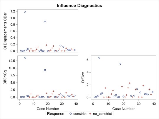
The index plots produced by the IPLOTS option are essentially the same line-printer plots as those produced by the INFLUENCE option, but with a 90-degree rotation and perhaps on a more refined scale. Since the ODS GRAPHICS ON statement is specified, the line-printer plots from the INFLUENCE and IPLOTS options are suppressed and ODS Graphics versions of the plots are displayed in Outputs 51.6.3 through 51.6.5. For general information about ODS Graphics, see Chapter 21, Statistical Graphics Using ODS. For specific information about the graphics available in the LOGISTIC procedure, see the section ODS Graphics. The vertical axis of an index plot represents the value of the diagnostic, and the horizontal axis represents the sequence (case number) of the observation. The index plots are useful for identification of extreme values.
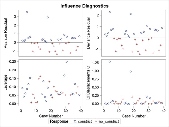
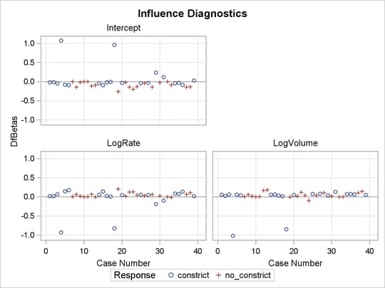
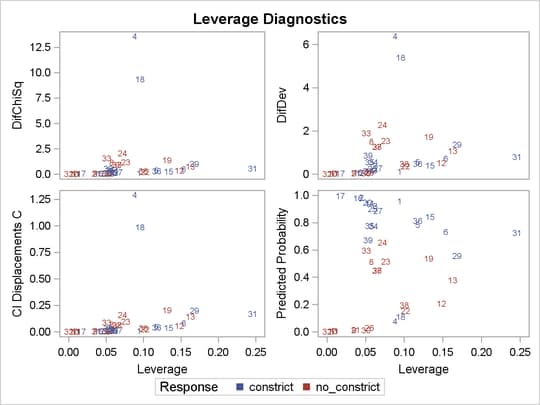
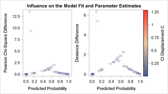
The index plots of the Pearson residuals and the deviance residuals (Output 51.6.3) indicate that case 4 and case 18 are poorly accounted for by the model. The index plot of the diagonal elements of the hat matrix (Output 51.6.3) suggests that case 31 is an extreme point in the design space. The index plots of DFBETAS (Output 51.6.5) indicate that case 4 and case 18 are causing instability in all three parameter estimates. The other four index plots in Outputs 51.6.3 and 51.6.4 also point to these two cases as having a large impact on the coefficients and goodness of fit.
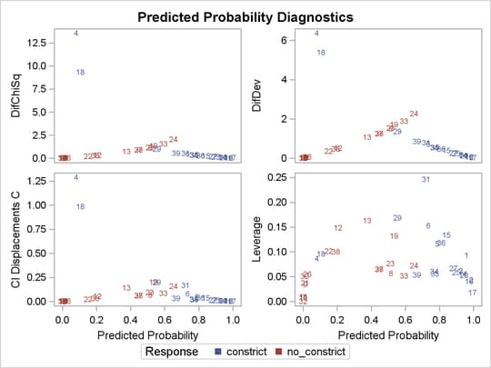
Other versions of diagnostic plots can be requested by specifying the appropriate options in the PLOTS= option. For example, the following statements produce three other sets of influence diagnostic plots: the PHAT option plots several diagnostics against the predicted probabilities (Output 51.6.6), the LEVERAGE option plots several diagnostics against the leverage (Output 51.6.7), and the DPC option plots the deletion diagnostics against the predicted probabilities and colors the observations according to the confidence interval displacement diagnostic (Output 51.6.8). The LABEL option displays the observation numbers on the plots. In all plots, you are looking for the outlying observations, and again cases 4 and 18 are noted.
ods graphics on;
proc logistic data=vaso plots(only label)=(phat leverage dpc);
   model Response=LogRate LogVolume;
run;
ods graphics off;
Copyright © SAS Institute, Inc. All Rights Reserved.