Example 37.9 Assessment of a Marginal Model for Dependent Data

This example illustrates the use of cumulative residuals to assess the adequacy of a marginal model for dependent data fit by generalized estimating equations (GEEs). The assessment methods are applied to CD4 count data from an AIDS clinical trial reported by Fischl, Richman, and Hansen (1990) and reanalyzed by Lin, Wei, and Ying (2002). The study randomly assigned 360 HIV patients to the drug AZT and 351 patients to placebo. CD4 counts were measured repeatedly over the course of the study. The data used here are the 4328 measurements taken in the first 40 weeks of the study.

The analysis focuses on the time trend of the response. The first model considered is

where is the time (in weeks) of the th measurement on the th patient, is the CD4 count at for the th patient, and is the indicator of AZT for the th patient. Normal errors and an independent working correlation are assumed.

The following statements create the SAS data set cd4:

data cd4;
   input Id Y Time Time2 TrtTime TrtTime2;
   Time3 = Time2 * Time;
   TrtTime3 = TrtTime2 * Time;
   datalines;
1     264.00024       -0.28571        0.08163       -0.28571        0.08163
1     175.00070        4.14286       17.16327        4.14286       17.16327
1     306.00150        8.14286       66.30612        8.14286       66.30612
1     331.99835       12.14286      147.44898       12.14286      147.44898
1     309.99929       16.14286      260.59184       16.14286      260.59184
1     185.00077       28.71429      824.51020       28.71429      824.51020
1     175.00070       40.14286     1611.44898       40.14286     1611.44898

   ... more lines ...   

711     488.00224       12.14286      147.44898       12.14286      147.44898
711     240.00026       18.14286      329.16327       18.14286      329.16327
;
run;

The following SAS statements fit the preceding model, create the cumulative residual plot in Output 37.9.1, and compute a -value for the model.

These graphical displays are requested by specifying the ODS GRAPHICS statement and the ASSESS statement. For general information about ODS Graphics, see Chapter 21, Statistical Graphics Using ODS. For specific information about the graphics available in the GENMOD procedure, see the section ODS Graphics.

Here, the SAS data set variables Time, Time2, TrtTime, and TrtTime2 correspond to , , , and , respectively. The variable Id identifies individual patients.

ods graphics on;
proc genmod data=cd4;
   class Id;
   model Y = Time Time2 TrtTime TrtTime2;
   repeated sub=Id;
   assess var=(Time) / resample
                       seed=603708000;
run;
ods graphics off;

Output 37.9.1 Cumulative Residual Plot for Quadratic Time Fit

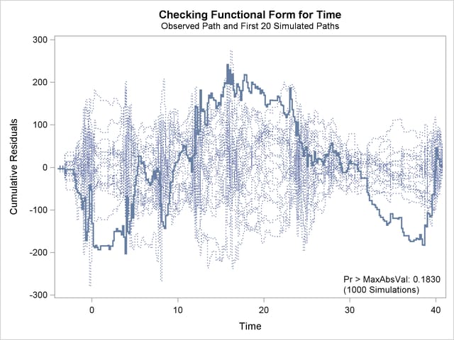
The cumulative residual plot in Output 37.9.1 displays cumulative residuals versus time for the model and 20 simulated realizations. The associated -value, also shown in Output 37.9.1, is 0.18. These results indicate that a more satisfactory model might be possible. The observed cumulative residual pattern most resembles plot (c) in Output 37.8.6, suggesting cubic time trends.

The following SAS statements fit the model, create the plot in Output 37.9.2, and compute a -value for a model with the additional terms and :

ods graphics on;
proc genmod data=cd4;
   class Id;
   model Y = Time Time2 Time3 TrtTime TrtTime2 TrtTime3;
   repeated sub=Id;
   assess var=(Time) / resample
                       seed=603708000;
run;
ods graphics off;

Output 37.9.2 Cumulative Residual Plot for Cubic Time Fit

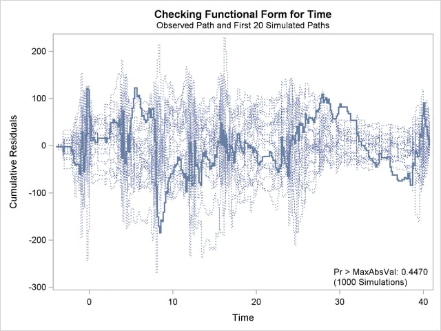
The observed cumulative residual pattern appears more typical of the simulated realizations, and the -value is 0.45, indicating that the model with cubic time trends is more appropriate.