| The GENMOD Procedure |
| Generalized Estimating Equations |
Let  ,
,  ,
,  , represent the
  th measurement on the
  th subject. There are
  measurements on subject and
  total measurements.
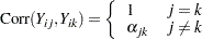
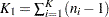
Correlated data are modeled using the same link function and linear predictor setup (systematic component) as the independence case. The random component is described by the same variance functions as in the independence case, but the covariance structure of the correlated measurements must also be modeled. Let the vector of measurements on the th subject be 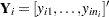 with corresponding vector of means
 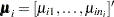 , and let
  be the covariance matrix of
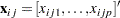
  . Let the vector of independent, or explanatory, variables for the th measurement on the th subject be
 |
The generalized estimating equation of Liang and Zeger (1986) for estimating the  vector of regression parameters
  is an extension of the independence estimating equation to correlated data and is given by
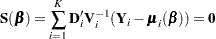 |
where
 |
Since
 |
where  is the link function, the
  matrix of partial derivatives of the mean with respect to the regression parameters for the th subject is given by
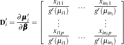 |
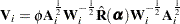
Working Correlation Matrix
Let  be an
be an  "working" correlation matrix that is fully specified by the vector of parameters
  . The covariance matrix of is modeled as
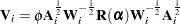 |
where  is an diagonal matrix with
  as the th diagonal element and
  is an diagonal matrix with
  as the th diagonal, where is a weight specified with the WEIGHT statement. If there is no WEIGHT statement,
  for all and . If is the true correlation matrix of , then is the true covariance matrix of .
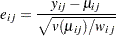
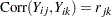
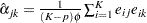
The working correlation matrix is usually unknown and must be estimated. It is estimated in the iterative fitting process by using the current value of the parameter vector to compute appropriate functions of the Pearson residual
 |
If you specify the working correlation as  , which is the identity matrix, the GEE reduces to the independence estimating equation.
Following are the structures of the working correlation supported by the GENMOD procedure and the estimators used to estimate the working correlations.
Working Correlation Structure |
Estimator |
|
|---|---|---|
Fixed |
||
|
The working correlation is not estimated in this case. |
|
Independent |
||
|
The working correlation is not estimated in this case. |
|
|
||
|
|
|
|
||
Exchangeable |
||
|
|
|
|
||
Unstructured |
||
|
|
|
Autoregressive AR(1) |
||
|
|
|
|
||
 where
where  is the
  th element of a constant, user-specified correlation matrix
  .
. 
 -dependent
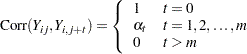
 for
for 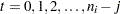
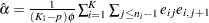
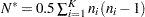
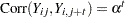
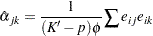
Dispersion Parameter
The dispersion parameter  is estimated by
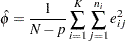 |
where  is the total number of measurements and
  is the number of regression parameters.
The square root of  is reported by PROC GENMOD as the scale parameter in the "Analysis of GEE Parameter Estimates Model-Based Standard Error Estimates" output table. If a fixed scale parameter is specified with the NOSCALE option in the MODEL statement, then the fixed value is used in estimating the model-based covariance matrix and standard errors.
Fitting Algorithm
The following is an algorithm for fitting the specified model by using GEEs. Note that this is not in general a likelihood-based method of estimation, so that inferences based on likelihoods are not possible for GEE methods.
Compute an initial estimate of
with an ordinary generalized linear model assuming independence. Compute the working correlations
 based on the standardized residuals, the current , and the assumed structure of .
 Compute an estimate of the covariance:
Update
: 
Repeat steps 2-4 until convergence.
Missing Data
See Diggle, Liang, and Zeger (1994, Chapter 11) for a discussion of missing values in longitudinal data. Suppose that you intend to take measurements  for the th unit. Missing values for which
  are missing whenever
  is missing for all
  are called dropouts. Otherwise, missing values that occur intermixed with nonmissing values are intermittent missing values. The GENMOD procedure can estimate the working correlation from data containing both types of missing values by using the all available pairs method, in which all nonmissing pairs of data are used in the moment estimators of the working correlation parameters defined previously. The resulting covariances and standard errors are valid under the missing completely at random (MCAR) assumption.
For example, for the unstructured working correlation model,
 |
where the sum is over the units that have nonmissing measurements at times and  , and
, and  is the number of units with nonmissing measurements at and . Estimates of the parameters for other working correlation types are computed in a similar manner, using available nonmissing pairs in the appropriate moment estimators.
The contribution of the th unit to the parameter update equation is computed by omitting the elements of  , the columns of
  , and the rows and columns of corresponding to missing measurements.
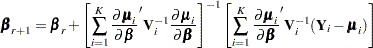
Parameter Estimate Covariances
The model-based estimator of  is given by
 |
where
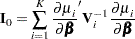 |
This is the GEE equivalent of the inverse of the Fisher information matrix that is often used in generalized linear models as an estimator of the covariance estimate of the maximum likelihood estimator of . It is a consistent estimator of the covariance matrix of  if the mean model and the working correlation matrix are correctly specified.
The estimator
 |
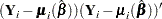
is called the empirical, or robust, estimator of the covariance matrix of , where
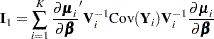 |
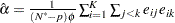
It has the property of being a consistent estimator of the covariance matrix of , even if the working correlation matrix is misspecified—that is, if  . See Zeger, Liang, and Albert (1988)), Royall (1986), and White (1982) for further information about the robust variance estimate. In computing
  , and are replaced by estimates, and
  is replaced by the estimate
 |
Multinomial GEEs
Lipsitz, Kim, and Zhao (1994) and Miller, Davis, and Landis (1993) describe how to extend GEEs to multinomial data. Currently, only the independent working correlation is available for multinomial models in PROC GENMOD.
Alternating Logistic Regressions
If the responses are binary (that is, they take only two values), then there is an alternative method to account for the association among the measurements. The alternating logistic regressions (ALR) algorithm of Carey, Zeger, and Diggle (1993) models the association between pairs of responses with log odds ratios, instead of with correlations, as ordinary GEEs do.
For binary data, the correlation between the jth and kth response is, by definition,
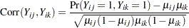 |
The joint probability in the numerator satisfies the following bounds, by elementary properties of probability, since 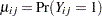 :
:
 |
The correlation, therefore, is constrained to be within limits that depend in a complicated way on the means of the data.
The odds ratio, defined as
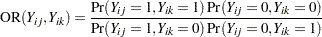 |
is not constrained by the means and is preferred, in some cases, to correlations for binary data.
The ALR algorithm seeks to model the logarithm of the odds ratio, 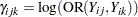 , as
, as
 |
where is a  vector of regression parameters and
  is a fixed, specified vector of coefficients.
The parameter  can take any value in
  with
with  corresponding to no association.
The log odds ratio, when modeled in this way with a regression model, can take different values in subgroups defined by . For example, can define subgroups within clusters, or it can define "block effects" between clusters.
You specify a GEE model for binary data that uses log odds ratios by specifying a model for the mean, as in ordinary GEEs, and a model for the log odds ratios. You can use any of the link functions appropriate for binary data in the model for the mean, such as logistic, probit, or complementary log-log. The ALR algorithm alternates between a GEE step to update the model for the mean and a logistic regression step to update the log odds ratio model. Upon convergence, the ALR algorithm provides estimates of the regression parameters for the mean, , the regression parameters for the log odds ratios, , their standard errors, and their covariances.
Specifying Log Odds Ratio Models
Specifying a regression model for the log odds ratio requires you to specify rows of the z matrix for each cluster and each unique within-cluster pair  . The GENMOD procedure provides several methods of specifying . These are controlled by the LOGOR=keyword and associated options in the REPEATED statement. The supported keywords and the resulting log odds ratio models are described as follows.
- EXCH
specifies exchangeable log odds ratios. In this model, the log odds ratio is a constant for all clusters
and pairs  . The parameter
  is the common log odds ratio.
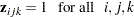
- FULLCLUST
specifies fully parameterized clusters. Each cluster is parameterized in the same way, and there is a parameter for each unique pair within clusters. If a complete cluster is of size
 , then there are
  parameters in the vector . For example, if a full cluster is of size 4, then there are
  parameters, and the z matrix is of the form
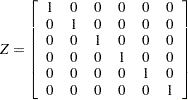
The elements of
correspond to log odds ratios for cluster pairs in the following order: Pair
Parameter
(1,2)
Alpha1
(1,3)
Alpha2
(1,4)
Alpha3
(2.3)
Alpha4
(2,4)
Alpha5
(3,4)
Alpha6
- LOGORVAR(variable)
specifies log odds ratios by cluster. The argument variable is a variable name that defines the "block effects" between clusters. The log odds ratios are constant within clusters, but they take a different value for each different value of the variable. For example, if Center is a variable in the input data set taking a different value for
treatment centers, then specifying LOGOR=LOGORVAR(Center) requests a model with different log odds ratios for each of the centers, constant within center. - NESTK
specifies k-nested log odds ratios. You must also specify the SUBCLUST=variable option to define subclusters within clusters. Within each cluster, PROC GENMOD computes a log odds ratio parameter for pairs having the same value of variable for both members of the pair and one log odds ratio parameter for each unique combination of different values of variable.
- NEST1
specifies 1-nested log odds ratios. You must also specify the SUBCLUST=variable option to define subclusters within clusters. There are two log odds ratio parameters for this model. Pairs having the same value of variable correspond to one parameter; pairs having different values of variable correspond to the other parameter. For example, if clusters are hospitals and subclusters are wards within hospitals, then patients within the same ward have one log odds ratio parameter, and patients from different wards have the other parameter.
- ZFULL
specifies the full z matrix. You must also specify a SAS data set containing the z matrix with the ZDATA=data-set-name option. Each observation in the data set corresponds to one row of the z matrix. You must specify the ZDATA data set as if all clusters are complete—that is, as if all clusters are the same size and there are no missing observations. The ZDATA data set has
 observations, where
  is the number of clusters and
  is the maximum cluster size. If the members of cluster are ordered as
  , then the rows of the z matrix must be specified for pairs in the order
  . The variables specified in the REPEATED statement for the SUBJECT effect must also be present in the ZDATA= data set to identify clusters. You must specify variables in the data set that define the columns of the z matrix by the ZROW=variable-list option. If there are
  columns ( variables in variable-list), then there are log odds ratio parameters. You can optionally specify variables indicating the cluster pairs corresponding to each row of the z matrix with the YPAIR=(variable1, variable2) option. If you specify this option, the data from the ZDATA data set are sorted within each cluster by variable1 and variable2. See Example 37.6 for an example of specifying a full z matrix.
 - ZREP
specifies a replicated z matrix. You specify z matrix data exactly as you do for the ZFULL case, except that you specify only one complete cluster. The z matrix for the one cluster is replicated for each cluster. The number of observations in the ZDATA data set is
 , where is the size of a complete cluster (a cluster with no missing observations).
 - ZREP(matrix)
specifies direct input of the replicated z matrix. You specify the z matrix for one cluster with the syntax LOGOR=ZREP (
 ), where
  and
and  are numbers representing a pair of observations and the values
  make up the corresponding row of the z matrix. The number of rows specified is , where is the size of a complete cluster (a cluster with no missing observations). For example,
 LOGOR = ZREP((1 2) 1 0, (1 3) 1 0, (1 4) 1 0, (2 3) 1 1, (2 4) 1 1, (3 4) 1 1)specifies the
rows of the z matrix for a cluster of size 4 with  log odds ratio parameters. The log odds ratio for the pairs (1 2), (1 3), (1 4) is
  , and the log odds ratio for the pairs (2 3), (2 4), (3 4) is
  .
.
Quasi-likelihood Information Criterion
The quasi-likelihood information criterion (QIC) was developed by Pan (2001) as a modification of the Akaike information criterion (AIC) to apply to models fit by GEEs.
Define the quasi-likelihood under the independence working correlation assumption, evaluated with the parameter estimates under the working correlation of interest as
 |
where the quasi-likelihood contribution of the th observation in the th cluster is defined in the section Quasi-likelihood Functions and  are the parameter estimates obtained from GEEs with the working correlation of interest
  .
.
QIC is defined as
 |
where  is the robust covariance estimate and
  is the inverse of the model-based covariance estimate under the independent working correlation assumption, evaluated at , the parameter estimates obtained from GEEs with the working correlation of interest .
PROC GENMOD also computes an approximation to  defined by Pan (2001) as
 |
where is the number of regression parameters.
Pan (2001) notes that QIC is appropriate for selecting regression models and working correlations, whereas  is appropriate only for selecting regression models.
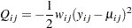
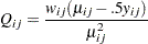
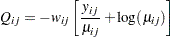
Quasi-likelihood Functions
See McCullagh and Nelder (1989) and Hardin and Hilbe (2003) for discussions of quasi-likelihood functions. The contribution of observation in cluster to the quasi-likelihood function evaluated at the regression parameters is given by 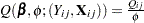 , where
  is defined in the following list. These are used in the computation of the quasi-likelihood information criteria (QIC) for goodness of fit of models fit with GEEs. The are prior weights, if any, specified with the WEIGHT or FREQ statements. Note that the definition of the quasi-likelihood for the negative binomial differs from that given in McCullagh and Nelder (1989). The definition used here allows the negative binomial quasi-likelihood to approach the Poisson as
  .
.
Normal:
Inverse Gaussian:
Gamma:
Negative binomial:

Poisson:
Binomial:

Multinomial (s categories):
Generalized Score Statistics
Boos (1992) and Rotnitzky and Jewell (1990) describe score tests applicable to testing  in GEEs, where
  is a user-specified
  contrast matrix or a contrast for a Type 3 test of hypothesis.
Let  be the regression parameters resulting from solving the GEE under the restricted model , and let
  be the generalized estimating equation values at .
The generalized score statistic is
 |
where  is the model-based covariance estimate and
  is the empirical covariance estimate. The p-values for
  are computed based on the chi-square distribution with r degrees of freedom.
Copyright © SAS Institute, Inc. All Rights Reserved.