The Power and Sample Size Application: Test of Mean Ratios

The Power and Sample Size Application

Test of Mean Ratios

Instead of comparing means for a control and drug treatment group, you might want to investigate whether the blood pressure of the treatment group is lowered by a given percentage of the control group, say 10 percent. That is, you expect the ratio of the treatment group to the control group to be 90% or less.

PSS provides a two-sample t test of a mean ratio when the data are lognormally distributed.

For mean ratios, the coefficient of variation (CV) is used instead of standard deviation. In this example, you can expect the CV to be between 0.5 and 0.6. You also want to compare an equally weighted sampling of groups with an overweighted sampling in which the control group contains twice as many subjects as the treatment group: 50 and 25, respectively.

Make a copy of the project by selecting File $\text{[math]}$ Save As. Enter a different project description, Percent improvement with blood pressure drug.

The copy of the project is opened.

Editing Properties

Several of the input parameters for the test of mean ratios differ from the ones described in the section Test of Two Independent Means for Equal Variances. Mean ratios and coefficients of variation are used instead of mean differences and standard deviations. These two parameters are discussed in detail in this section. For the input parameters and options that have been discussed previously in this example, only the values for this example are given.

Solve For Tab

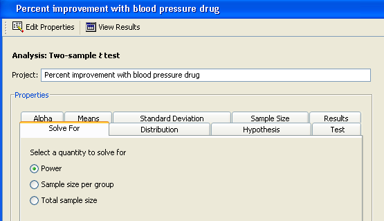
Click the Solve For tab to select the Power option as the quantity to be solved for, as shown in Figure 69.49.

Figure 69.49 Project Description, Solve for Tab

Distribution

You are interested in mean ratios rather than means, so select the Lognormal option on the Distribution tab, as shown in Figure 69.50.

Figure 69.50 Distribution Tab with Lognormal Option

Hypothesis and Alpha

Click the Hypothesis tab and select the One-sided test option.

Click the Alpha tab and type 0.05 as the significance level in the first cell of the table, if it is not already there.

Means

Click the Means tab to select the input form for entering mean ratios. There are four alternate forms for entering means or mean ratios:

Mean ratio: Enter the ratio of the two group means—that is, the treatment mean divided by the reference mean. The null ratio is assumed to be 1.
Group means: Enter the means for each group. The ratio of the means is formed by dividing the mean for group 2 by the mean for group 1. The null ratio is assumed to be 1.
Mean ratio, Null ratio: Enter the ratio of the two group means—that is, the treatment mean divided by the reference mean. Enter the null ratio.
Group means, Null ratio: Enter the means for each group. The ratio of the means is formed by dividing the mean for group 2 by the mean for group 1. Enter the null ratio.

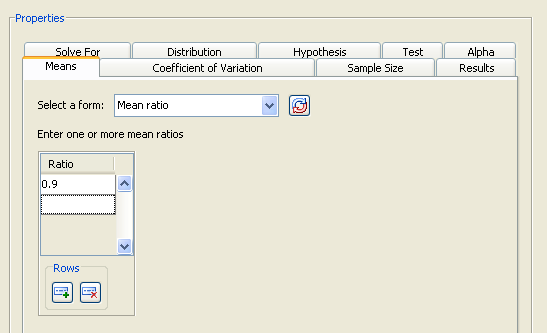
As shown in Figure 69.51, select the Mean ratio form which uses a default null ratio of 1. Enter a single mean ratio value of 0.9.

Figure 69.51 Means Tab with Mean Ration Form and Values

Coefficient of Variation

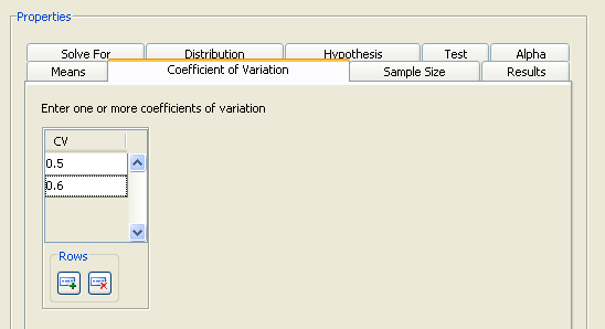
On the Coefficient of Variation tab, enter the coefficients of variation. They are assumed to be equal for the two groups.

For this example, enter 0.5 and 0.6, as shown in Figure 69.52.

Figure 69.52 Coefficient of Variation Tab

Sample Size

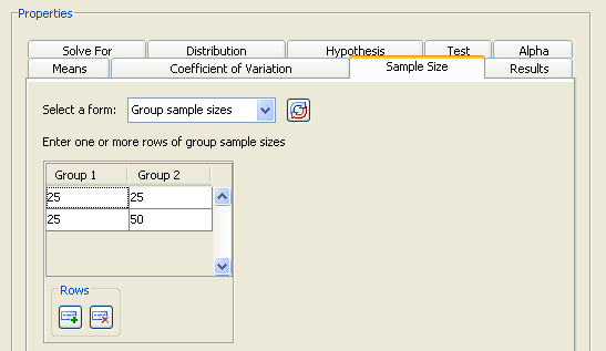
On the Sample Size tab, select the Group sample sizes form and enter two sets of values: 25 and 25 in the first row and 25 and 50 in the second row, as shown in Figure 69.53.

Figure 69.53 Sample Sizes

Summary of Input Parameters

Table 69.4 contains the values of the input parameters for the example.

Table 69.4 Summary of Input Parameters
Parameter	Value
Hypothesis	One-sided test
Distribution	Lognormal
Alpha	0.05
Means form	Mean ratio
Mean ratio	0.9
Coefficients of variation	0.5, 0.6
Sample size form	Group sample sizes
Sample Size	(25, 25), (25, 50)

Results

On the Results tab, select the Create summary table and Create power by sample size graph check boxes.

Click Calculate to perform the analysis.

In this case, the following message is displayed:

The power by sample size graph is not available when specifying sample sizes for two groups.

If you want a power by sample size graph, you can choose to plot total sample size instead by using the Total N, Group weights sample size form on the Sample Size tab. For more information about using this input form, see the section Using Unequal Group Sizes.

Viewing Results

The first thing that you notice from the summary table in Figure 69.54 is that the calculated powers are quite low—they range from 0.163 to 0.229. You have less than a 25% probability of detecting the difference that you are looking for. Clearly, this set of parameter values leads to insufficient power. To increase power, you might choose a larger sample size or a larger alpha.

Figure 69.54 Summary Table

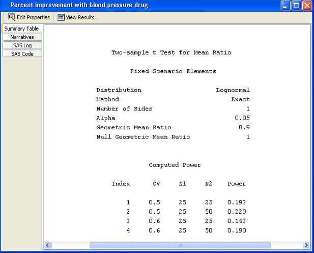
You can also see that oversampling the control group improves power slightly, 0.229 versus 0.193 for the coefficient of variation of 0.5. However, this is a marginal increase that is probably not worth the added expense.

For the example, use larger sample sizes with equal cell sizes. Return to the Edit Properties page by clicking the Edit Properties icon near the top of the window.

Then, on the Sample size tab, change to the Sample size per group form. Specify sample sizes of 50, 100, 150, and 200, as shown in Figure 69.55.

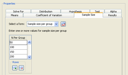
Figure 69.55 Modified Sample Size Values

Table 69.5 contains the modified values of the input parameters for the example.

Table 69.5 Modified Summary of Input Parameters
Parameter	Value
Sample size form	Sample size per group
Sample size	50, 100, 150, 200

Rerun the analysis by clicking Calculate.

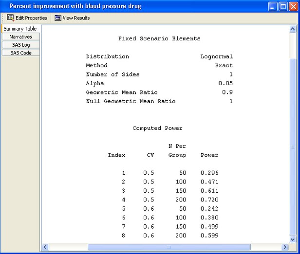
Figure 69.56 displays the summary table. The largest sample size of 200 (per group) yields a power of 0.72 for a coefficient of variation of 0.5, and 0.599 for one of 0.6. With a total of 400 subjects, you still have a 30% to 40% probability of not detecting the effect even if it exists.

Figure 69.56 Summary Table for Modified Sample Sizes

Top of Page