| The TCALIS Procedure |
Example 88.9 Linear Relations among Factor Loadings
In this example, a confirmatory factor-analysis model with linear constraints on loadings is specified by the FACTOR modeling language of PROC TCALIS. SAS programming statements are used to set the constraints. In the context of the current example, the differences between fitting covariance structures and correlation structures will also be discussed.
The correlation matrix of six variables from Kinzer and Kinzer (N=326) is used by Guttman (1957) as an example that yields an approximate simplex. McDonald (1980) uses this data set as an example of factor analysis where he assumes that the loadings on the second factor are linear functions of the loadings on the first factor. Let  be the factor loading matrix containing the two factors and six variables so that:
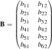 |
and
 |
The correlation structures are represented by:
 |
where  represents the diagonal matrix of unique variances for the variables.
With parameters  and
and  being unconstrained, McDonald (1980) has fitted an underidentified model with seven degrees of freedom. Browne (1982) imposes the following identification condition:
 |
In this example, Browne’s identification condition is imposed. The following is the specification of the confirmatory factor model using the FACTOR modeling language.
   data kinzer(type=corr);
   title "Data Matrix of Kinzer & Kinzer, see GUTTMAN (1957)";
      _type_ = 'corr';
      input _name_ $ var1-var6;
      datalines;
   var1  1.00   .     .     .     .     .
   var2   .51  1.00   .     .     .     .
   var3   .46   .51  1.00   .     .     .
   var4   .46   .47   .54  1.00   .     .
   var5   .40   .39   .49   .57  1.00   .
   var6   .33   .39   .47   .45   .56  1.00
     ;
   proc tcalis data=kinzer nobs=326 nose;
      factor
         factor1 -> var1-var6 = b11 b21 b31 b41 b51 b61 (6 *.6),
         factor2 -> var1-var6 = b12 b22 b32 b42 b52 b62;
      pvar
         factor1-factor2 = 2 * 1.,
         var1-var6       = psi1-psi6 (6 *.3);
      parameters alpha (1.);
      /* SAS Programming Statements to define dependent parameters */
      b12 = alpha - b11;
      b22 = alpha - b21;
      b32 = alpha - b31;
      b42 = alpha - b41;
      b52 = alpha - b51;
      b62 = alpha - b61;
      fitindex on(only)=[chisq df probchi];
   run;
In the FACTOR statement, you specify two factors, named factor1 and factor2, for the variables. In this model, all manifest variables have nonzero loadings on the two factors. These loading parameters are specified after the equal signs and are named with the prefix 'b.' Initial estimates are given in the parentheses. For example, in the first entry of factor-variable relations, you specify loadings of var1–var6 on factor1. All these loadings are free parameters and are given the same initial value  . Loadings of var1–var6 on factor2 are also defined as parameters in the same statement. However, they are dependent parameters because they are functionally dependent on other independent parameters, as shown in the SAS programming statements afterwards. Initial values for these dependent parameters are thus unnecessary.
In the PVAR statement, the factor variances are fixed at ones, while the error variances for the variables are free parameters named psi1–psi6. Again, initial estimates are provided in the parentheses that follow after the parameter names.
An additional parameter alpha is specified in the PARAMETERS statement with an initial value of 1. Then, six SAS programming statements are used to define the loadings on the second factor as functions of the loadings on the first factor. Lastly, the FITINDEX statement is used to trim the results in the fit summary table.
In the specification, there are twelve loadings in the FACTOR statement and six unique variances in the PVAR statement. Adding the parameter alpha in the list, there are 19 parameters in total. However, the loading parameters are not all independent of each other. As defined in the SAS programming statements, six loadings are dependent. This reduces the number of free parameters to 13. Hence the degrees of freedom for the model is  . Notice that the factor variances are fixed at 1 and covariances among factors are fixed zeros by default.
In Output 88.9.1, a concise fit summary table is shown. The chi-square test statistic of model fit is 10.337 with  =8 (
=8 ( =0.242). This indicates a good model fit.
The estimated factor loading matrix is presented in Output 88.9.2, and the estimated error variances and the estimate for alpha are presented in Output 88.9.3.
All these estimates are essentially the same as reported in Browne (1982). Notice that there are no standard error estimates in the output, as requested by the NOSE option in the PROC TCALIS statement. Standard error estimates are not of interest in this example.
In fitting the preceding factor model, wrong covariance structures rather than the intended correlation structures have been specified. As pointed out by Browne (1982), fitting such covariance structures directly is not entirely appropriate for analyzing correlations. For example, when fitting the correlation structures, the diagonal elements of  must always be fixed ones. This fact has never been enforced in the preceding specification. A simple check of the estimates will illustrate the problem. In Output 88.9.2, the loading estimates of VAR1 on the two factors are
  and
and  , respectively. In Output 88.9.3, the error variance estimate for VAR1 is
  . The fitted variance of VAR1 can therefore be computed by the following equation:
 |
This fitted value is quite a bit off from 1.00, as required for the standardized variance of VAR1.
Fortunately, even though the wrong covariance structure model has been analyzed, the preceding analysis is not completely useless. For the current confirmatory factor model, according to Browne (1982) the estimates obtained from fitting the wrong covariance structure model are still consistent (as if they were estimating the population parameters in the correlation structures). However, the chi-square test statistic as reported previously is not correct.
Note that using the CORR option in the PROC TCALIS statement will not solve the problem. By specifying the CORR option you merely request PROC TCALIS to use the correlation matrix directly as a covariance matrix in the objective function for model fitting. It still would not constrain the fitting of the diagonal elements to 1 during estimation.
In the next section, a solution to the stated problem is suggested. It is not claimed that this is the only solution or the best solution. Alternative treatments of the problem are possible.
Fitting the Correct Correlation Structures
This main idea of this solution is to embed the intended correlation structures (with correct constraints on the diagonal elements of the correlation matrix) into a covariance structure model so that the estimation methods of PROC TCALIS can be applied legitimately to the specially constructed covariance structures.
First, the issue of the fixed ones on the diagonal of the correlation structure model is addressed. That is, the diagonal elements of the correlation structures represented by  must be fitted by ones. This can be accomplished by constraining the error variances as dependent parameters of the loadings, as shown in the following:
 |
Other constraints might also serve the purpose, but the ones just presented are the most convenient and intuitive.
Now, due to the fact that discrepancy functions used in PROC TCALIS are derived for covariance matrices rather than correlation matrices, PROC TCALIS is essentially set up for analyzing covariance structures (with or without mean structures), but not correlation structures. Hence, the statistical theory behind PROC TCALIS applies to covariance structure analysis, but it might not generalize to correlation structure analysis in all situations. Despite that, with some manipulations PROC TCALIS can fit the correct correlation structures to the current data without compromising the statistical theory. These manipulations are now discussed. Recall that the correlation structures are represented by:
|
As before, in the matrix, there are six linear constraints on the factor loadings. In addition, the diagonal elements of are constrained to ones, as done by defining the error variances as dependent parameters of the loadings in the preceding equation. To analyze the correlation structures by using PROC TCALIS, a covariance structure model with such correlation structures embedded is now specified. That is, the covariance structure to be fitted by PROC TCALIS is as follows:
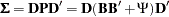 |
where  is a 6 x 6 diagonal matrix containing the population standard deviations for the manifest variables. Theoretically, it is legitimate that you analyze this covariance structure model for studying the embedded correlation structures. In addition, it does not matter whether your input matrix is a correlation or covariance matrix, or any rescaled covariance matrix (by multiplying any variables by any positive constants). You would get correct results if you could somehow specify these covariance structures correctly in PROC TCALIS. However, there seems to be nowhere in PROC TCALIS that you can specify the diagonal matrix for the population standard deviations. So what can one do with this formulation? The answer is to rewrite the covariance structure model in a form similar to the usual confirmatory factor model, as presented in the following.
Let  and
and  . The covariance structure model of interest can now be rewritten as:
 |
This form of covariance structures implies a confirmatory factor model with factor loading matrix  and error covariance matrix
  . This confirmatory factor model can certainly be specified using the FACTOR modeling language, in much the same way you specify a confirmatory factor model in the preceding section. However, because you are actually more interested in estimating the basic set of parameters in matrices and
  of the embedded correlation structures, you would define the model parameters as functions of this basic set of parameters of interest. This can be accomplished by using the PARAMETERS and the SAS programming statements.
All in all, you can use the following statements to set up such a confirmatory factor model with the desired correlation structures embedded.
   proc tcalis data=Kinzer nobs=326 nose;
      factor
         factor1 -> var1-var6 = t11 t21 t31 t41 t51 t61,
         factor2 -> var1-var6 = t12 t22 t32 t42 t52 t62;
      pvar
         factor1-factor2 = 2 * 1.,
         var1-var6       = k1-k6;
      parameters alpha (1.) d1-d6 (6 * 1.)
                 b11 b21 b31 b41 b51 b61 (6 *.6),
                 b12 b22 b32 b42 b52 b62
                 psi1-psi6;
      /* SAS Programming Statements */
      /* 12 Constraints on Correlation structures */
      b12  = alpha - b11;
      b22  = alpha - b21;
      b32  = alpha - b31;
      b42  = alpha - b41;
      b52  = alpha - b51;
      b62  = alpha - b61;
      psi1 = 1. - b11 * b11 - b12 * b12;
      psi2 = 1. - b21 * b21 - b22 * b22;
      psi3 = 1. - b31 * b31 - b32 * b32;
      psi4 = 1. - b41 * b41 - b42 * b42;
      psi5 = 1. - b51 * b51 - b52 * b52;
      psi6 = 1. - b61 * b61 - b62 * b62;
      /* Defining Covariance Structure Parameters */
      t11  = d1 * b11;
      t21  = d2 * b21;
      t31  = d3 * b31;
      t41  = d4 * b41;
      t51  = d5 * b51;
      t61  = d6 * b61;
      t12  = d1 * b12;
      t22  = d2 * b22;
      t32  = d3 * b32;
      t42  = d4 * b42;
      t52  = d5 * b52;
      t62  = d6 * b62;
      k1   = d1 * d1 * psi1;
      k2   = d2 * d2 * psi2;
      k3   = d3 * d3 * psi3;
      k4   = d4 * d4 * psi4;
      k5   = d5 * d5 * psi5;
      k6   = d6 * d6 * psi6;
      fitindex on(only)=[chisq df probchi];
   run;
First, you notice that specifications in the FACTOR and the PVAR statements are essentially unchanged from the previous specification, except that the parameters are named differently here to reflect different model matrices. In the current specification, the factor loading parameters in matrix are named with prefix 't,' and the error variance parameters in matrix are named with prefix 'k.' Specification of these parameters reflects the covariance structures. As you see in the last block of the SAS programming statements statements, all these parameters are functions of the correlation structure parameters in , , and .
Next, in the PARAMETERS statement, all correlation structure parameters are defined with initial values provided. These are the parameters of interest: alpha is used to define dependencies among loadings, d’s are the population standard deviations, b’s are the loading parameters, and psi’s are the error variance parameters. There are 25 parameters specified in this statement, but not all of them are free or independent.
In the first block of SAS programming statements, parameter dependencies or constraints on the correlation structures are specified. The first six statements realize the required linear relations among the factor loadings:
 |
The next six statements constrain the error variances so as to ensure that an embedded correlation structure model is being fitted. That is, each error variance is dependent on the corresponding loadings, as prescribed by the following equation:
|
These twelve constraints reduce the number of independent parameters to 13, as expected.
The next block of SAS programming statements are essentially for relating the correlation structure parameters to the covariance structures that are specified in the FACTOR and the PVAR statements. These SAS programming statements realize the required relations: and , but in non-matrix forms:
 |
 |
where  denotes the j-th diagonal element of .
The fit summary is presented in Output 88.9.4. The chi-square test statistic is 14.63 with =8 (=0.067). This shows that the previous chi-square test based on fitting a wrong covariance structure model is indeed questionable.
Estimates of the loadings and error variances are presented in Output 88.9.5. These estimates are for the covariance structure model with loading matrix and error covariance matrix . They are rescaled versions of the correlation structure parameters and are not of primary interest themselves.
The parameter estimates of the embedded correlation structures are shown in Output 88.9.6 as "additional" parameters.
| Additional Parameters | ||
|---|---|---|
| Type | Parameter | Estimate |
| Independent | alpha | 0.97400 |
| d1 | 1.00771 | |
| d2 | 0.99712 | |
| d3 | 0.99078 | |
| d4 | 0.99085 | |
| d5 | 0.99640 | |
| d6 | 1.01687 | |
| b11 | 0.34217 | |
| b21 | 0.32095 | |
| b31 | 0.49179 | |
| b41 | 0.57553 | |
| b51 | 0.77686 | |
| b61 | 0.66659 | |
| Dependent | b12 | 0.63183 |
| b22 | 0.65305 | |
| b32 | 0.48222 | |
| b42 | 0.39848 | |
| b52 | 0.19714 | |
| b62 | 0.30742 | |
| psi1 | 0.48371 | |
| psi2 | 0.47051 | |
| psi3 | 0.52561 | |
| psi4 | 0.50998 | |
| psi5 | 0.35762 | |
| psi6 | 0.46116 | |
Except for the population standard deviation parameter d’s, all other parameters estimated in the current model can be compared with those from the previous fitting of an incorrect covariance structure model. Although estimates in the current model do not differ very much from those in the previous specification, it is at least reassuring that they are obtained from fitting a correctly specified covariance structure model with the intended correlation structures embedded.
Note: This procedure is experimental.
Copyright © 2009 by SAS Institute Inc., Cary, NC, USA. All rights reserved.