| The SEQTEST Procedure |
Getting Started: SEQTEST Procedure
The following example illustrates a clinical study that uses a two-sided O’Brien-Fleming design (O’Brien and Fleming 1979) to stop the trial early for ethical concerns about possible harm or for unexpectedly strong efficacy of the new drug.
Suppose that a pharmaceutical company is conducting a clinical trial to test the efficacy of a new cholesterol-lowering drug. The primary focus is low-density lipoprotein (LDL), the so-called bad cholesterol, which is a risk factor for coronary heart disease. LDL is measured in  , milligrams per deciliter of blood.
The trial consists of two groups of equally allocated patients with elevated LDL level: an experimental group given the new drug and a placebo control group. Suppose the changes in LDL level after the treatment for patients in the experimental and control groups are normally distributed with means  and
and  , respectively, and have a common variance
  . Then the null hypothesis of no effect for the new drug is
 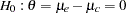 . Also suppose that the alternative reference
  is the clinically meaningful difference that the trial should detect with a high probability (power), and that a good estimate of the standard deviation for the changes in LDL level is
  .
.
The following statements invoke the SEQDESIGN procedure and request a four-stage O’Brien-Fleming design for standardized normal test statistics:
   ods graphics on;
   proc seqdesign altref=-10.0;
     TwoSidedOBrienFleming: design nstages=4
                            method=obf
                            ;
     samplesize model=twosamplemean(stddev=20);
     ods output Boundary=Bnd_LDL;
   run;
   ods graphics off;
The ALTREF= option specifies the alternative reference, and the actual maximum information is derived in the SEQDESIGN procedure.
In the DESIGN statement, the label TwoSidedOBrienFleming identifies the design in the output tables. The default ALT=TWOSIDED option specifies a two-sided alternative hypothesis. The default STOP=REJECT option specifies early stopping in the interim stages only for the purpose of rejecting the null hypothesis. That is, at each interim stage, the trial will either be stopped to reject the null hypothesis or continue to the next stage.
The NSTAGES= option in the DESIGN statement specifies the total number of stages in the group sequential trial, including three interim stages and a final stage. In the SEQDESIGN procedure, the null hypothesis for the design is
  . The default ALPHA=0.05 option specifies a Type I error probability
  , and the default BETA=0.10 option specifies a Type II error probability
  , which corresponds to a power of
  at the alternative reference
  .
.
For a two-sided design with early stopping to reject the null hypothesis, there are two boundaries for the design: an upper  (rejection) boundary that consists of upper rejection critical values and a lower boundary that consists of lower rejection critical values. Each boundary is a set of critical values, one from each stage. With the METHOD=OBF option in the DESIGN statement, the O’Brien-Fleming method is used for the two boundaries for the design; see Figure 78.5.
The SAMPLESIZE statement with the MODEL=TWOSAMPLEMEAN option uses the derived maximum information to compute required sample sizes for a two-sample test for mean difference.
The ODS OUTPUT statement with the BOUNDARY=BND_LDL option creates an output data set named BND_LDL which contains the resulting boundary information. At each stage of the trial, data are collected and analyzed with a statistical procedure, and a test statistic and its corresponding information level are computed.
In this example, you can use the REG procedure to compute the maximum likelihood estimate  for the drug effect and the corresponding standard error for . At stage
  , you can use the SEQTEST procedure to compare the test statistic with adjusted boundaries that are derived from the boundary information stored in the BOUND_LDL data set. At each subsequent stage, you can use the SEQTEST procedure to compare the test statistic with adjusted boundaries that are derived from the boundary information stored in the test information table that was created by the SEQTEST procedure at the previous stage. The test information tables are structured for input to the SEQTEST procedure.
At each interim stage, the trial will either be stopped to reject the null hypothesis or continue to the next stage. At the final stage, the null hypothesis is either rejected or accepted.
By default, the SEQDESIGN procedure derives boundary values with equally spaced information levels for all stages—that is, the same information increment between successive stages.
The "Design Information" table in Figure 78.3 displays design specifications and three derived statistics: the maximum information, the average sample number under the null hypothesis (Null Ref ASN), and the average sample number under the alternative hypothesis (Alt Ref ASN). Each statistic is expressed as a percentage of the identical statistic for the corresponding fixed-sample information. The average sample number is the expected sample size (for nonsurvival data) or expected number of events (for survival data). When you specify an alternative reference (in this case, ALTREF= ), the actual maximum information
  is also computed. Note that for a symmetric two-sided design, the ALTREF= option implies a lower alternative reference of and an upper alternative reference of
  .
.
| Design Information | |
|---|---|
| Statistic Distribution | Normal |
| Boundary Scale | Standardized Z |
| Alternative Hypothesis | Two-Sided |
| Early Stop | Reject Null |
| Method | O'Brien-Fleming |
| Boundary Key | Both |
| Alternative Reference | -10 |
| Number of Stages | 4 |
| Alpha | 0.05 |
| Beta | 0.1 |
| Power | 0.9 |
| Max Information (Percent of Fixed Sample) | 102.2163 |
| Max Information | 0.107403 |
| Null Ref ASN (Percent of Fixed Sample) | 101.5728 |
| Alt Ref ASN (Percent of Fixed Sample) | 76.7397 |
The "Boundary Information" table in Figure 78.4 displays the information level, the lower and upper alternative references, and the lower and upper boundary values at each stage. By default, the SEQDESIGN procedure uses equally spaced information levels for all stages.
| Boundary Information (Standardized Z Scale) Null Reference = 0 |
|||||||
|---|---|---|---|---|---|---|---|
| _Stage_ | Alternative | Boundary Values | |||||
| Information Level | Reference | Lower | Upper | ||||
| Proportion | Actual | N | Lower | Upper | Alpha | Alpha | |
| 1 | 0.2500 | 0.026851 | 42.96116 | -1.63862 | 1.63862 | -4.04859 | 4.04859 |
| 2 | 0.5000 | 0.053701 | 85.92233 | -2.31736 | 2.31736 | -2.86278 | 2.86278 |
| 3 | 0.7500 | 0.080552 | 128.8835 | -2.83817 | 2.83817 | -2.33745 | 2.33745 |
| 4 | 1.0000 | 0.107403 | 171.8447 | -3.27724 | 3.27724 | -2.02429 | 2.02429 |
The information proportion is the proportion of maximum information available at each stage. With the BOUNDARYSCALE=STDZ option, the alternative references and boundary values are displayed with the standardized  statistic scale. The alternative reference in the standardized scale at stage
  is given by
  , where
  is the alternative reference and
  is the information available at stage ,
  .
.
In this example, a standardized statistic is computed by standardizing the parameter estimate of the effect in LDL level. A lower test statistic indicates a beneficial effect. Consequently, at each interim stage, if the standardized test statistic is less than or equal to the corresponding lower boundary value, the hypothesis is rejected for efficacy. If the test statistic is greater than or equal to the corresponding upper boundary value, the hypothesis  is rejected for harmful effect. Otherwise, the process continues to the next stage. At the final stage (stage ), the hypothesis is rejected for efficacy if the statistic is less than or equal to the corresponding lower boundary value
  , and the hypothesis is rejected for harmful effect if the statistic is greater than or equal to the corresponding upper boundary value
  . Otherwise, the hypothesis of no significant difference is accepted.
Note that in a typical trial, the actual information levels do not match the information levels specified in the design. Consequently, the SEQTEST procedure modifies the boundary values stored in the BND_LDL data set to adjust for these new information levels.
If the ODS GRAPHICS ON statement is specified, a detailed boundary plot with the rejection and acceptance regions is displayed by default, as shown in Figure 78.5.
This boundary plot displays the boundary values in the "Boundary Information" table in Figure 78.4. The stages are indicated by vertical lines with accompanying stage numbers. The horizontal axis indicates the information levels for the stages. If a test statistic at an interim stage is in the rejection region (shaded area), the trial stops and the null hypothesis is rejected. If the statistic is not in any rejection region, the trial continues to the next stage. The plot also displays critical values for the corresponding fixed-sample design. The symbol " " identifies the fixed-sample critical values of
  and
and  .
.
When you specify the SAMPLESIZE statement, the maximum information (either explicitly specified or derived in the SEQDESIGN procedure) is used to compute the required sample sizes for the study. The MODEL=TWOSAMPLEMEAN(STDDEV=20) option specifies the test for the difference between two normal means. See the section "Test for the Difference between Two Normal Means" in the chapter "The SEQDESIGN Procedure" for a detailed description of how these required sample sizes are calculated.
The "Sample Size Summary" table in Figure 78.6 displays the parameters for the sample size computation and the resulting maximum and expected sample sizes.
With the derived maximum information and the specified MODEL=TWOSAMPLEMEAN
(STDDEV=20) option in the SAMPLESIZE statement, the total sample size in each group is
 |
The "Sample Sizes (N)" table in Figure 78.7 displays the required sample sizes at each stage for the trial, in both fractional and integer numbers. The derived fractional sample sizes are displayed under the heading "Fractional N." These sample sizes are rounded up to integers under the heading "Ceiling N." With the default WEIGHT=1 option in the SAMPLESIZE statement, the sample sizes for the two groups are equal for the two-sample test.
| Sample Sizes (N) Two-Sample Z Test for Mean Difference |
||||||||
|---|---|---|---|---|---|---|---|---|
| _Stage_ | Fractional N | Ceiling N | ||||||
| N | N(Grp 1) | N(Grp 2) | Information | N | N(Grp 1) | N(Grp 2) | Information | |
| 1 | 42.96 | 21.48 | 21.48 | 0.0269 | 44 | 22 | 22 | 0.0275 |
| 2 | 85.92 | 42.96 | 42.96 | 0.0537 | 86 | 43 | 43 | 0.0538 |
| 3 | 128.88 | 64.44 | 64.44 | 0.0806 | 130 | 65 | 65 | 0.0812 |
| 4 | 171.84 | 85.92 | 85.92 | 0.1074 | 172 | 86 | 86 | 0.1075 |
In practice, integer sample sizes are used in the trial, and the resulting information levels increase slightly. Thus, each of the two groups needs  ,
,  ,
,  , and
, and  patients for the four stages, respectively.
Suppose that patients are available in each group at stage and that their measurements for LDL are saved in the data set LDL_1. Figure 78.8 lists the first 10 observations in the data set LDL_1.
The variable Trt is an indicator variable with value for patients in the treatment group and value  for patients in the placebo control group. The variable Ldl is the LDL level of these patients.
The following statements use the REG procedure to estimate the mean treatment difference and its associated standard error at stage :
   proc reg data=LDL_1;
      model Ldl=Trt;
   ods output ParameterEstimates=Parms_LDL1;
   run;
The following statements create the data set for the mean treatment difference and its associated standard error as a PARMS= data set, which will subsequently serve as an input data set for PROC SEQTEST. Note that all of the variables are required for a PARMS= data set, as described in the section PARMS < (TESTVAR= variable) > = SAS Data Set.
   data Parms_LDL1;
      set Parms_LDL1;
      if Variable='Trt';
      _Scale_='MLE';
      _Stage_= 1;
      keep _Scale_ _Stage_ Variable Estimate StdErr;
   run;

   proc print data=Parms_LDL1;
      title 'Statistics Computed at Stage 1';
   run;
Figure 78.9 displays the statistics computed at stage .
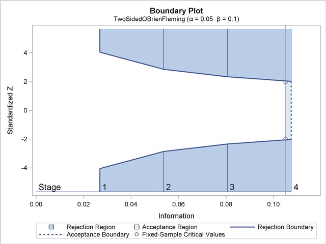
Since the sample sizes derived are based on the estimated variance at the designing phase, the information level that corresponds to the test statistic at stage is estimated by
 |
where  is the standard error of the treatment estimate.
The following statements invoke the SEQTEST procedure to test for early stopping at stage :
   ods graphics on;
   proc seqtest Boundary=Bnd_LDL
                Parms(Testvar=Trt)=Parms_LDL1
                ;
   ods output Test=Test_LDL1;
   run;
   ods graphics off;
The BOUNDARY= option specifies the input data set that provides the boundary information for the trial at stage , which was generated in the SEQDESIGN procedure. The PARMS=PARMS_LDL1 option specifies the input data set PARMS_LDL1 that contains the test statistic and its associated standard error at stage , and the TESTVAR=TRT option identifies the test variable TRT in the data set.
The ODS OUTPUT statement with the TEST=TEST_LDL1 option creates an output data set named TEST_LDL1 which contains the updated boundary information for the test at stage . The data set also provides the boundary information that is needed for the group sequential test at the next stage. See the section Boundary Adjustments for Information Levels for details.
The "Design Information" table in Figure 78.10 displays design specifications. By default, the boundary values are modified for the updated information levels to maintain the Type I level. The maximum information remains the same as in the original design, but the derived Type II error probability  and power
  are slightly different with new information levels. With the updated power , the corresponding fixed-sample design is also updated.
| Design Information | |
|---|---|
| BOUNDARY Data Set | WORK.BND_LDL |
| Data Set | WORK.PARMS_LDL1 |
| Statistic Distribution | Normal |
| Boundary Scale | Standardized Z |
| Alternative Hypothesis | Two-Sided |
| Early Stop | Reject Null |
| Number of Stages | 4 |
| Alpha | 0.05 |
| Beta | 0.10074 |
| Power | 0.89926 |
| Max Information (Percent of Fixed Sample) | 102.4815 |
| Max Information | 0.10740291 |
| Null Ref ASN (Percent of Fixed Sample) | 101.7765 |
| Alt Ref ASN (Percent of Fixed Sample) | 75.4928 |
The "Test Information" table in Figure 78.11 displays the boundary values for the test statistic with the default standardized scale. Since only the information level at stage is available from the PARMS= data set, information levels at future interim stages are derived proportionally from the corresponding information levels in the original design.
| Test Information (Standardized Z Scale) Null Reference = 0 |
||||||||
|---|---|---|---|---|---|---|---|---|
| _Stage_ | Alternative | Boundary Values | Test | |||||
| Information Level | Reference | Lower | Upper | Trt | ||||
| Proportion | Actual | Lower | Upper | Alpha | Alpha | Estimate | Action | |
| 1 | 0.2880 | 0.030934 | -1.75879 | 1.75879 | -3.39532 | 3.39532 | -0.44426 | Continue |
| 2 | 0.5253 | 0.056423 | -2.37536 | 2.37536 | -2.77374 | 2.77374 | . | |
| 3 | 0.7627 | 0.081913 | -2.86205 | 2.86205 | -2.32412 | 2.32412 | . | |
| 4 | 1.0000 | 0.107403 | -3.27724 | 3.27724 | -2.03147 | 2.03147 | . | |
At stage , the standardized statistic  is between the lower and upper boundary values, and so the trial continues to the next stage. With the observed information level at stage ,
  (which is not substantially different from the target information level at stage ), the trial continues to the next stage without adjustment of the sample size according to the study plan.
Note that if an observed information level is different from its target level at an interim stage, the sample sizes at future stages might be adjusted to achieve the target maximum information level according to the study plan. For example, a study plan might modify the final sample size to achieve the target maximum information level if the observed information level is different from its target level by a specified amount at the interim stage. If the variance estimate is used to compute the required sample size for the group sequential trial, the study plan might use the current variance estimate to update the required sample size for the trial (Jennison and Turnbull 2000, p. 295).
If the ODS GRAPHICS ON statement is specified, a detailed test plot with the rejection and acceptance regions is displayed by default, as shown in Figure 78.12. This plot displays the boundary values in the "Test Information" table in Figure 78.11. The stages are indicated by vertical lines with accompanying stage numbers. The horizontal axis indicates the information levels for the stages. As expected, the test statistic is in the continuation region between the lower and upper boundaries.

The following statements use the REG procedure with the data available at the first two stages to estimate the mean treatment difference and its associated standard error at stage  :
:
   proc reg data=LDL_2;
      model Ldl=Trt;
   ods output ParameterEstimates=Parms_LDL2;
   run;
The following statements create and display (in Figure 78.13) the data set for the mean treatment difference and its associated standard error:
   data Parms_LDL2;
      set Parms_LDL2;
      if Variable='Trt';
      _Scale_='MLE';
      _Stage_= 2;
      keep _Scale_ _Stage_ Variable Estimate StdErr;
   run;

   proc print data=Parms_LDL2;
      title 'Statistics Computed at Stage 2';
   run;
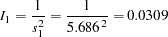
Using the standard error for the treatment estimate available at stage , the information level that corresponds to the test statistic at stage is estimated by
 |
where  is the standard error of the treatment estimate at stage .
The following statements invoke the SEQTEST procedure to test for early stopping at stage :
   proc seqtest Boundary=Test_LDL1
                Parms(Testvar=Trt)=Parms_LDL2
                ;
   ods output Test=Test_LDL2;
   run;
The BOUNDARY= option specifies the input data set that provides the boundary information for the trial at stage , which was generated by the SEQTEST procedure at the previous stage. The PARMS= option specifies the input data set that contains the test statistic and its associated standard error at stage , and the TESTVAR= option identifies the test variable in the data set.
The ODS OUTPUT statement with the TEST=TEST_LDL2 option creates an output data set named TEST_LDL2 which contains the updated boundary information for the test at stage . The data set also provides the boundary information that is needed for the group sequential test at the next stage.
The "Test Information" table in Figure 78.14 displays the boundary values for the test statistic with the default standardized scale.
| Test Information (Standardized Z Scale) Null Reference = 0 |
||||||||
|---|---|---|---|---|---|---|---|---|
| _Stage_ | Alternative | Boundary Values | Test | |||||
| Information Level | Reference | Lower | Upper | Trt | ||||
| Proportion | Actual | Lower | Upper | Alpha | Alpha | Estimate | Action | |
| 1 | 0.2880 | 0.030934 | -1.75879 | 1.75879 | -3.39532 | 3.39532 | -0.44426 | Continue |
| 2 | 0.5169 | 0.055519 | -2.35624 | 2.35624 | -2.78456 | 2.78456 | -1.97365 | Continue |
| 3 | 0.7585 | 0.081461 | -2.85413 | 2.85413 | -2.32908 | 2.32908 | . | |
| 4 | 1.0000 | 0.107403 | -3.27724 | 3.27724 | -2.03097 | 2.03097 | . | |
At stage , the standardized test statistic,  , is between its corresponding lower and upper boundary values. Therefore, the trial continues to the next stage.
The following statements use the REG procedure with the data available at the first three stages to estimate the mean treatment difference and its associated standard error at stage  :
:
   proc reg data=LDL_3;
      model Ldl=Trt;
   ods output ParameterEstimates=Parms_LDL3;
   run;
The following statements create and display (in Figure 78.15) the data set for the mean treatment difference and its associated standard error:
   data Parms_LDL3;
      set Parms_LDL3;
      if Variable='Trt';
      _Scale_='MLE';
      _Stage_= 3;
      keep _Scale_ _Stage_ Variable Estimate StdErr;
   run;

   proc print data=Parms_LDL3;
      title 'Statistics Computed at Stage 3';
   run;
The following statements invoke the SEQTEST procedure to test for early stopping at stage :
   ods graphics on;
   proc seqtest Boundary=Test_LDL2
                Parms(Testvar=Trt)=Parms_LDL3
                ;
   ods output Test=Test_LDL3;
   run;
   ods graphics off;
The BOUNDARY= option specifies the input data set that provides the boundary information for the trial at stage , which was generated by the SEQTEST procedure at the previous stage. The PARMS= option specifies the input data set that contains the test statistic and its associated standard error at stage , and the TESTVAR= option identifies the test variable in the data set.
The ODS OUTPUT statement with the TEST=TEST_LDL3 option creates an output data set named TEST_LDL3 which contains the updated boundary information for the test at stage . The data set also provides the boundary information that is needed for the group sequential test at the next stage.
The "Test Information" table in Figure 78.16 displays the boundary values for the test statistic with the default standardized scale.
| Test Information (Standardized Z Scale) Null Reference = 0 |
||||||||
|---|---|---|---|---|---|---|---|---|
| _Stage_ | Alternative | Boundary Values | Test | |||||
| Information Level | Reference | Lower | Upper | Trt | ||||
| Proportion | Actual | Lower | Upper | Alpha | Alpha | Estimate | Action | |
| 1 | 0.2880 | 0.030934 | -1.75879 | 1.75879 | -3.39532 | 3.39532 | -0.44426 | Continue |
| 2 | 0.5169 | 0.055519 | -2.35624 | 2.35624 | -2.78456 | 2.78456 | -1.97365 | Continue |
| 3 | 0.7953 | 0.085422 | -2.92271 | 2.92271 | -2.25480 | 2.25480 | -2.69289 | Reject Null |
| 4 | 1.0000 | 0.107403 | -3.27724 | 3.27724 | -2.04573 | 2.04573 | . | |
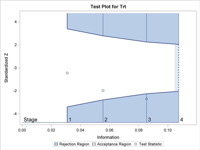
The sequential test stops at stage to reject the null hypothesis for the lower alternative because the test statistic  is less than the corresponding upper boundary
  . That is, the test demonstrates significant beneficial effect for the new drug.
The "Test Plot" displays boundary values for the design and the test statistic at the first three stages, as shown in Figure 78.17. It shows that the test statistic is in the "Rejection Region" below the lower boundary at stage .
When a trial stops, the "Parameter Estimates" table in Figure 78.18 displays the stopping stage, parameter estimate, unbiased median estimate, confidence limits, and  -value under the null hypothesis . As expected, the -value
  is significant at the two-sided level,
  , and the confidence interval does not contain the value zero. The -value, unbiased median estimate, and confidence limits depend on the ordering of the sample space
  , where is the stage number and
  is the standardized statistic. See the section Analysis after a Sequential Test for a detailed description of these statistics.
Copyright © 2009 by SAS Institute Inc., Cary, NC, USA. All rights reserved.