PROC NLMIXED: Nonlinear Growth Curves with Gaussian Data :: SAS/STAT(R) 9.2 User's Guide, Second Edition

The NLMIXED Procedure

Nonlinear Growth Curves with Gaussian Data

As an introductory example, consider the orange tree data of Draper and Smith (1981). These data consist of seven measurements of the trunk circumference (in millimeters) on each of five orange trees. You can input these data into a SAS data set as follows:

   data tree;
     input tree day y;
     datalines;
   1  118   30
   1  484   58
   1  664   87
   1 1004  115
   1 1231  120
   1 1372  142
   1 1582  145
   2  118   33
   2  484   69
   2  664  111
   2 1004  156
   2 1231  172
   2 1372  203
   2 1582  203
   3  118   30
   3  484   51
   3  664   75
   3 1004  108
   3 1231  115
   3 1372  139
   3 1582  140
   4  118   32
   4  484   62
   4  664  112
   4 1004  167
   4 1231  179
   4 1372  209
   4 1582  214
   5  118   30
   5  484   49
   5  664   81
   5 1004  125
   5 1231  142
   5 1372  174
   5 1582  177
   ;

Lindstrom and Bates (1990) and Pinheiro and Bates (1995) propose the following logistic nonlinear mixed model for these data:

$\text{[math]}$

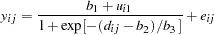Here, $\text{[math]}$ represents the $\text{[math]}$ th measurement on the $\text{[math]}$ th tree ( $\text{[math]}$ ; $\text{[math]}$ ), $\text{[math]}$ is the corresponding day, $\text{[math]}$ are the fixed-effects parameters, $\text{[math]}$ are the random-effect parameters assumed to be iid $\text{[math]}$ , and $\text{[math]}$ are the residual errors assumed to be iid $\text{[math]}$ and independent of the $\text{[math]}$ . This model has a logistic form, and the random-effect parameters $\text{[math]}$ enter the model linearly.

The statements to fit this nonlinear mixed model are as follows:

   proc nlmixed data=tree;
      parms b1=190 b2=700 b3=350 s2u=1000 s2e=60;
      num = b1+u1;
      ex  = exp(-(day-b2)/b3);
      den = 1 + ex;
      model y ~ normal(num/den,s2e);
      random u1 ~ normal(0,s2u) subject=tree;
   run;

The PROC NLMIXED statement invokes the procedure and inputs the tree data set. The PARMS statement identifies the unknown parameters and their starting values. Here there are three fixed-effects parameters (b1, b2, b3) and two variance components (s2u, s2e).

The next three statements are SAS programming statements specifying the logistic mixed model. A new variable u1 is included to identify the random effect. These statements are evaluated for every observation in the data set when the NLMIXED procedure computes the log likelihood function and its derivatives.

The MODEL statement defines the dependent variable and its conditional distribution given the random effects. Here a normal (Gaussian) conditional distribution is specified with mean num/den and variance s2e.

The RANDOM statement defines the single random effect to be u1, and specifies that it follow a normal distribution with mean 0 and variance s2u. The SUBJECT= argument in the RANDOM statement defines a variable indicating when the random effect obtains new realizations; in this case, it changes according to the values of the tree variable. PROC NLMIXED assumes that the input data set is clustered according to the levels of the tree variable; that is, all observations from the same tree occur sequentially in the input data set.

The output from this analysis is as follows.

Figure 61.1 Model Specifications

The NLMIXED Procedure

Specifications
Data Set	WORK.TREE
Dependent Variable	y
Distribution for Dependent Variable	Normal
Random Effects	u1
Distribution for Random Effects	Normal
Subject Variable	tree
Optimization Technique	Dual Quasi-Newton
Integration Method	Adaptive Gaussian Quadrature

The "Specifications" table lists basic information about the nonlinear mixed model you have specified (Figure 61.1). Included are the input data set, the dependent and subject variables, the random effects, the relevant distributions, and the type of optimization. The "Dimensions" table lists various counts related to the model, including the number of observations, subjects, and parameters (Figure 61.2). These quantities are useful for checking that you have specified your data set and model correctly. Also listed is the number of quadrature points that PROC NLMIXED has selected based on the evaluation of the log likelihood at the starting values of the parameters. Here, only one quadrature point is necessary because the random-effect parameters $\text{[math]}$ enter the model linearly. (The Gauss-Hermite quadrature with a single quadrature point results in the Laplace approximation of the log likelihood.)

Figure 61.2 Dimensions Table for Growth Curve Model

Dimensions
Observations Used	35
Observations Not Used	0
Total Observations	35
Subjects	5
Max Obs Per Subject	7
Parameters	5
Quadrature Points	1

Figure 61.3 Starting Values of Parameter Estimates and Negative Log Likelihood

Parameters
b1	b2	b3	s2u	s2e	NegLogLike
190	700	350	1000	60	132.491787

The "Parameters" table lists the parameters to be estimated, their starting values, and the negative log likelihood evaluated at the starting values (Figure 61.3).

Figure 61.4 Iteration History for Growth Curve Model

Iteration History
Iter	Calls	NegLogLike	Diff	MaxGrad	Slope
1	4	131.686742	0.805045	0.010269	-0.633
2	6	131.64466	0.042082	0.014783	-0.0182
3	8	131.614077	0.030583	0.009809	-0.02796
4	10	131.572522	0.041555	0.001186	-0.01344
5	11	131.571895	0.000627	0.0002	-0.00121
6	13	131.571889	5.549E-6	0.000092	-7.68E-6
7	15	131.571888	1.096E-6	6.097E-6	-1.29E-6

NOTE: GCONV convergence criterion satisfied.

The "Iteration History" table records the history of the minimization of the negative log likelihood (Figure 61.4). For each iteration of the quasi-Newton optimization, values are listed for the number of function calls, the value of the negative log likelihood, the difference from the previous iteration, the absolute value of the largest gradient, and the slope of the search direction. The note at the bottom of the table indicates that the algorithm has converged successfully according to the GCONV convergence criterion, a standard criterion computed using a quadratic form in the gradient and the inverse Hessian.

The final maximized value of the log likelihood as well as the information criterion of Akaike (AIC), its small sample bias corrected version (AICC), and the Bayesian information criterion (BIC) in the "smaller is better" form appear in the "Fit Statistics" table (Figure 61.5). These statistics can be used to compare different nonlinear mixed models.

Figure 61.5 Fit Statistics for Growth Curve Model

Fit Statistics
-2 Log Likelihood	263.1
AIC (smaller is better)	273.1
AICC (smaller is better)	275.2
BIC (smaller is better)	271.2

Figure 61.6 Parameter Estimates at Convergence

Parameter Estimates
Parameter	Estimate	Standard Error	DF	t Value	Pr > \|t\|	Alpha	Lower	Upper	Gradient
b1	192.05	15.6473	4	12.27	0.0003	0.05	148.61	235.50	1.154E-6
b2	727.90	35.2472	4	20.65	<.0001	0.05	630.04	825.76	5.289E-6
b3	348.07	27.0790	4	12.85	0.0002	0.05	272.88	423.25	-6.1E-6
s2u	999.88	647.44	4	1.54	0.1974	0.05	-797.70	2797.45	-3.84E-6
s2e	61.5139	15.8831	4	3.87	0.0179	0.05	17.4153	105.61	2.892E-6

The maximum likelihood estimates of the five parameters and their approximate standard errors computed using the final Hessian matrix are displayed in the "Parameter Estimates" table (Figure 61.6). Approximate $\text{[math]}$ -values and Wald-type confidence limits are also provided, with degrees of freedom equal to the number of subjects minus the number of random effects. You should interpret these statistics cautiously for variance parameters like s2u and s2e. The final column in the output shows the gradient vector at the optimization solution. Each element appears to be sufficiently small to indicate a stationary point.

Since the random-effect parameters $\text{[math]}$ enter the model linearly, you can obtain equivalent results by using the first-order method (specify METHOD=FIRO in the PROC NLMIXED statement).

Top of Page