| The MCMC Procedure |
Example 52.9 Normal Regression with Interval Censoring
You can use PROC MCMC to fit failure time data that can be right, left, or interval censored. To illustrate, a normal regression model is used in this example.
Assume that you have the following simple regression model with no covariates:
 |
where  is a vector of response values (the failure times),
  is the grand mean,
  is an unknown scale parameter, and
  are errors from the standard normal distribution. Instead of observing
  directly, you only observe a truncated value
  . If the true occurs after the censored time , it is called right censoring. If occurs before the censored time, it is called left censoring. A failure time can be censored at both ends, and this is called interval censoring. The likelihood for is as follows:
 |
where  is the survival function,
 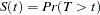 .
.
Gentleman and Geyer (1994) uses the following data on cosmetic deterioration for early breast cancer patients treated with radiotherapy:
   title 'Normal Regression with Interval Censoring';
   data cosmetic;
      label tl = 'Time to Event (Months)';
      input tl tr @@;
      datalines;
   45  .   6 10   .  7  46  .  46  .   7 16  17  .   7 14
   37 44   .  8   4 11  15  .  11 15  22  .  46  .  46  .
   25 37  46  .  26 40  46  .  27 34  36 44  46  .  36 48
   37  .  40  .  17 25  46  .  11 18  38  .   5 12  37  .
    .  5  18  .  24  .  36  .   5 11  19 35  17 25  24  .
   32  .  33  .  19 26  37  .  34  .  36  .
   ;
The data consist of time interval endpoints (in months). Nonmissing equal endpoints (tl = tr) indicates uncensoring; a nonmissing lower endpoint (tl  .) and a missing upper endpoint (tr = .) indicates right censoring; a missing lower endpoint (tl = .) and a nonmissing upper endpoint (tr .) indicates left censoring; and nonmissing unequal endpoints (tl tr) indicates interval censoring.
With this data set, you can consider using proper but diffuse priors on both and , for example:
 |
 |
 |
|||
 |
|
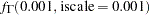 |
where  is the gamma density function.
The following SAS statements fit an interval censoring model and generate Output 52.9.1:
   proc mcmc data=cosmetic outpost=postout seed=1 nmc=20000 missing=AC;
      ods select PostSummaries PostIntervals;
      parms mu 60 sigma 50;

      prior mu ~ normal(0, sd=1000);
      prior sigma ~ gamma(shape=0.001,iscale=0.001);

      if (tl^=. and tr^=. and tl=tr) then
         llike = logpdf('normal',tr,mu,sigma);
      else if (tl^=. and tr=.) then
         llike = logsdf('normal',tl,mu,sigma);
      else if (tl=. and tr^=.) then
         llike = logcdf('normal',tr,mu,sigma);
      else
         llike = log(sdf('normal',tl,mu,sigma) -
            sdf('normal',tr,mu,sigma));

      model general(llike);
   run;
Because there are missing cells in the input data, you want to use the MISSING=AC option so that PROC MCMC does not delete any observations that contain missing values. The IF-ELSE statements distinguish different censoring cases for , according to the likelihood. The SAS functions LOGCDF, LOGSDF, LOGPDF, and SDF are useful here. The MODEL statement assigns llike as the log likelihood to the response. The Markov chain appears to have converged in this example (evidence not shown here), and the posterior estimates are shown in Output 52.9.1.
| Posterior Summaries | ||||||
|---|---|---|---|---|---|---|
| Parameter | N | Mean | Standard Deviation |
Percentiles | ||
| 25% | 50% | 75% | ||||
| mu | 20000 | 41.7807 | 5.7882 | 37.7220 | 41.3468 | 45.2249 |
| sigma | 20000 | 29.1122 | 6.0503 | 24.8774 | 28.2210 | 32.4250 |
Copyright © 2009 by SAS Institute Inc., Cary, NC, USA. All rights reserved.