| The LOGISTIC Procedure |
Example 51.8 Comparing Receiver Operating Characteristic Curves
DeLong, DeLong, and Clarke-Pearson (1988) report on 49 patients with ovarian cancer who also suffer from an intestinal obstruction. Three (correlated) screening tests are measured to determine whether a patient will benefit from surgery. The three tests are the K-G score and two measures of nutritional status: total protein and albumin. The data are as follows:
   data roc;
      input alb tp totscore popind @@;
      totscore = 10 - totscore;
      datalines;
   3.0 5.8 10 0   3.2 6.3  5 1   3.9 6.8  3 1   2.8 4.8  6 0
   3.2 5.8  3 1   0.9 4.0  5 0   2.5 5.7  8 0   1.6 5.6  5 1
   3.8 5.7  5 1   3.7 6.7  6 1   3.2 5.4  4 1   3.8 6.6  6 1
   4.1 6.6  5 1   3.6 5.7  5 1   4.3 7.0  4 1   3.6 6.7  4 0
   2.3 4.4  6 1   4.2 7.6  4 0   4.0 6.6  6 0   3.5 5.8  6 1
   3.8 6.8  7 1   3.0 4.7  8 0   4.5 7.4  5 1   3.7 7.4  5 1
   3.1 6.6  6 1   4.1 8.2  6 1   4.3 7.0  5 1   4.3 6.5  4 1
   3.2 5.1  5 1   2.6 4.7  6 1   3.3 6.8  6 0   1.7 4.0  7 0
   3.7 6.1  5 1   3.3 6.3  7 1   4.2 7.7  6 1   3.5 6.2  5 1
   2.9 5.7  9 0   2.1 4.8  7 1   2.8 6.2  8 0   4.0 7.0  7 1
   3.3 5.7  6 1   3.7 6.9  5 1   3.6 6.6  5 1
   ;
In the following statements, the NOFIT option is specified in the MODEL statement to prevent PROC LOGISTIC from fitting the model with three covariates. Each ROC statement lists one of the covariates, and PROC LOGISTIC then fits the model with that single covariate. Note that the original data set contains six more records with missing values for one of the tests, but PROC LOGISTIC ignores all records with missing values; hence there is a common sample size for each of the three models. The ROCCONTRAST statement implements the nonparameteric approach of DeLong, DeLong, and Clarke-Pearson (1988) to compare the three ROC curves, the REFERENCE option specifies that the K-G Score curve is used as the reference curve in the contrast, the E option displays the contrast coefficients, and the ESTIMATE option computes and tests each comparison. The ODS GRAPHICS statement and the plots=roc(id=prob) specification in the PROC LOGISTIC statement will display several plots, and the plots of individual ROC curves will have certain points labeled with their predicted probabilities.
   ods graphics on;
   proc logistic data=roc plots=roc(id=prob);
      model popind(event='0') = alb tp totscore / nofit;
      roc 'Albumin' alb;
      roc 'K-G Score' totscore;
      roc 'Total Protein' tp;
      roccontrast reference('K-G Score') / estimate e;
   run;
   ods graphics off;
The initial model information is displayed in Output 51.8.1.
For each ROC model, the model fitting details in Outputs 51.8.2, 51.8.4, and 51.8.6 can be suppressed with the ROCOPTIONS(NODETAILS) option; however, the convergence status is always displayed.
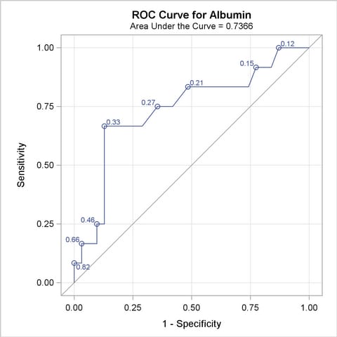
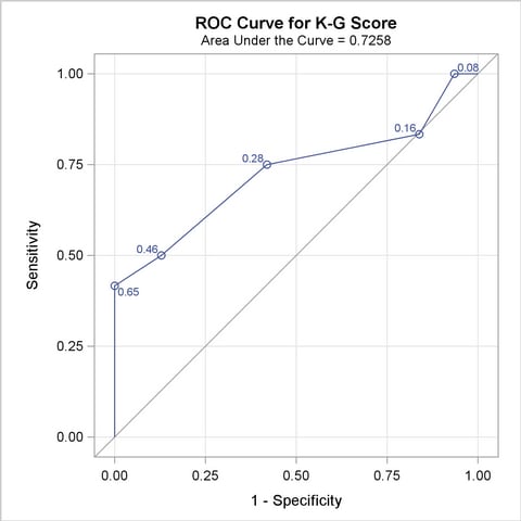
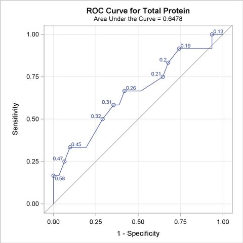
The ROC curves for the three models are displayed in Outputs 51.8.3, 51.8.5, and 51.8.7. Note that the labels on the ROC curve are produced by specifying the ID=PROB option, and are the predicted probabilities for the cutpoints.
| Model Fit Statistics | ||
|---|---|---|
| Criterion | Intercept Only |
Intercept and Covariates |
| AIC | 52.918 | 49.384 |
| SC | 54.679 | 52.907 |
| -2 Log L | 50.918 | 45.384 |
| Testing Global Null Hypothesis: BETA=0 | |||
|---|---|---|---|
| Test | Chi-Square | DF | Pr > ChiSq |
| Likelihood Ratio | 5.5339 | 1 | 0.0187 |
| Score | 5.6893 | 1 | 0.0171 |
| Wald | 4.6869 | 1 | 0.0304 |
| Model Fit Statistics | ||
|---|---|---|
| Criterion | Intercept Only |
Intercept and Covariates |
| AIC | 52.918 | 46.262 |
| SC | 54.679 | 49.784 |
| -2 Log L | 50.918 | 42.262 |
| Testing Global Null Hypothesis: BETA=0 | |||
|---|---|---|---|
| Test | Chi-Square | DF | Pr > ChiSq |
| Likelihood Ratio | 8.6567 | 1 | 0.0033 |
| Score | 8.3613 | 1 | 0.0038 |
| Wald | 6.3845 | 1 | 0.0115 |
| Model Fit Statistics | ||
|---|---|---|
| Criterion | Intercept Only |
Intercept and Covariates |
| AIC | 52.918 | 51.794 |
| SC | 54.679 | 55.316 |
| -2 Log L | 50.918 | 47.794 |
| Testing Global Null Hypothesis: BETA=0 | |||
|---|---|---|---|
| Test | Chi-Square | DF | Pr > ChiSq |
| Likelihood Ratio | 3.1244 | 1 | 0.0771 |
| Score | 3.1123 | 1 | 0.0777 |
| Wald | 2.9059 | 1 | 0.0883 |
All ROC curves being compared are also overlaid on the same plot, as shown in Output 51.8.8.
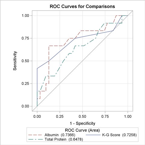
Output 51.8.9 displays the association statistics, and displays the area under the ROC curve (estimated by "c" in the "ROC Association Statistics" table) along with its standard error and a confidence interval for each model in the comparison. The confidence interval for Total Protein contains 0.50; hence it is not significantly different from random guessing, which is represented by the diagonal line in the preceding ROC plots.
| ROC Association Statistics | |||||||
|---|---|---|---|---|---|---|---|
| ROC Model | Mann-Whitney | Somers' D (Gini) |
Gamma | Tau-a | |||
| Area | Standard Error |
95% Wald Confidence Limits |
|||||
| Albumin | 0.7366 | 0.0927 | 0.5549 | 0.9182 | 0.4731 | 0.4809 | 0.1949 |
| K-G Score | 0.7258 | 0.1028 | 0.5243 | 0.9273 | 0.4516 | 0.5217 | 0.1860 |
| Total Protein | 0.6478 | 0.1000 | 0.4518 | 0.8439 | 0.2957 | 0.3107 | 0.1218 |
Output 51.8.10 shows that the contrast used ’K-G Score’ as the reference level. This table is produced by specifying the E option in the ROCCONTRAST statement.
Output 51.8.11 shows that the 2-degrees-of-freedom test that the ’K-G Score’ is different from at least one other test is not significant at the 0.05 level.
Output 51.8.12 is produced by specifying the ESTIMATE option. Each row shows that the curves are not significantly different.
Copyright © 2009 by SAS Institute Inc., Cary, NC, USA. All rights reserved.