| Introduction to Structural Equation Modeling with Latent Variables |
Some Measurement Models
Psychometric test theory involves many kinds of models relating scores on psychological and educational tests to latent variables representing intelligence or various underlying abilities. The following example uses data on four vocabulary tests from Lord (1957). Tests  and
and  have 15 items each and are administered with very liberal time limits. Tests
  and
and  have 75 items and are administered under time pressure. The covariance matrix is read by the following DATA step:
   data lord(type=cov);
      input _type_ $ _name_ $ w x y z;
      datalines;
   n   . 649       .       .       .
   cov w 86.3979   .       .       .
   cov x 57.7751 86.2632   .       .
   cov y 56.8651 59.3177 97.2850   .
   cov z 58.8986 59.6683 73.8201 97.8192
   ;
The psychometric model of interest states that and are determined by a single common factor  , and and are determined by a single common factor
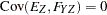
  . The two common factors are expected to have a positive correlation, and it is desired to estimate this correlation. It is convenient to assume that the common factors have unit variance, so their correlation will be equal to their covariance. The error terms for all the manifest variables are assumed to be uncorrelated with each other and with the common factors. The model (labeled here as model form D) is as follows.
Model Form D
 |
 |
 |
|||
 |
|
 |
|||
 |
|
 |
|||
 |
|
 |
with the following assumptions:
 |
|
 |
|||
 |
|
 |
|||
 |
|
 |
|||
 |
|
 |
|||
|
|
 |
|||
|
|
 |
|||
|
|
 |
The corresponding path diagram is shown in Figure 17.10.
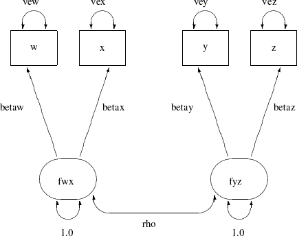
With the following rules, the conversion from the path diagram to the PATH model specification is very straightforward:
Each single-headed arrow in the path diagram is specified in the PATH statement.
Each double-headed arrow that points to a single variable is specified in the PVAR statement.
Each double-headed arrow that points to two distinct variables is specified in the PCOV statement.
Hence, this path diagram can be converted easily to a PATH model as follows:
   title 'H4: Unconstrained';
   proc tcalis data=lord outmodel=model4;
      path
         w <- fwx    betaw,
         x <- fwx    betax,
         y <- fyz    betay,
         z <- fyz    betaz;
      pvar
         fwx fyz = 2 * 1.0,
         w x y z = vew vex vey vez;
      pcov
         fwx fyz = rho;
   run;
The major results are displayed in Figure 17.11 and Figure 17.12.
| Fit Summary | ||
|---|---|---|
| Modeling Info | N Observations | 649 |
| N Variables | 4 | |
| N Moments | 10 | |
| N Parameters | 9 | |
| N Active Constraints | 0 | |
| Independence Model Chi-Square | 1466.5524 | |
| Independence Model Chi-Square DF | 6 | |
| Absolute Index | Fit Function | 0.0011 |
| Chi-Square | 0.7030 | |
| Chi-Square DF | 1 | |
| Pr > Chi-Square | 0.4018 | |
| Z-Test of Wilson & Hilferty | 0.2363 | |
| Hoelter Critical N | 3543 | |
| Root Mean Square Residual (RMSR) | 0.2720 | |
| Standardized RMSR (SRMSR) | 0.0030 | |
| Goodness of Fit Index (GFI) | 0.9995 | |
| Parsimony Index | Adjusted GFI (AGFI) | 0.9946 |
| Parsimonious GFI | 0.1666 | |
| RMSEA Estimate | 0.0000 | |
| RMSEA Lower 90% Confidence Limit | . | |
| RMSEA Upper 90% Confidence Limit | 0.0974 | |
| Probability of Close Fit | 0.6854 | |
| ECVI Estimate | 0.0291 | |
| ECVI Lower 90% Confidence Limit | . | |
| ECVI Upper 90% Confidence Limit | 0.0391 | |
| Akaike Information Criterion | -1.2970 | |
| Bozdogan CAIC | -6.7725 | |
| Schwarz Bayesian Criterion | -5.7725 | |
| McDonald Centrality | 1.0002 | |
| Incremental Index | Bentler Comparative Fit Index | 1.0000 |
| Bentler-Bonett NFI | 0.9995 | |
| Bentler-Bonett Non-normed Index | 1.0012 | |
| Bollen Normed Index Rho1 | 0.9971 | |
| Bollen Non-normed Index Delta2 | 1.0002 | |
| James et al. Parsimonious NFI | 0.1666 | |
| PATH List | ||||||
|---|---|---|---|---|---|---|
| Path | Parameter | Estimate | Standard Error |
t Value | ||
| w | <- | fwx | betaw | 7.50066 | 0.32339 | 23.19390 |
| x | <- | fwx | betax | 7.70266 | 0.32063 | 24.02354 |
| y | <- | fyz | betay | 8.50947 | 0.32694 | 26.02730 |
| z | <- | fyz | betaz | 8.67505 | 0.32560 | 26.64301 |
It is convenient to create the OUTMODEL= data set called model4 for use in fitting other models with additional constraints. The same analysis can be performed with the LINEQS statement, as specified in the following:
   title 'H4: Unconstrained; LINEQS Specification';
   proc tcalis data=lord;
      lineqs w = betaw fwx + ew,
             x = betax fwx + ex,
             y = betay fyz + ey,
             z = betaz fyz + ez;
      std fwx fyz = 2 * 1.,
          ew ex ey ez = vew vex vey vez;
      cov fwx fyz = rho;
   run;
Unlike the PATH model specification, in the LINEQS specification you need to specify the error terms explicitly in the LINEQS statement. In the STD statement, you would need to specify the variance parameters for the exogenous variables, including both of the factors and the error terms. However, using the PATH model specification, no explicit names for error or disturbance terms are needed. As a result, the exogenous variance and error variance parameters are both specified in the PVAR statement. This treatment generalizes to the following useful rule about the PATH model specification:
Each variable in the PATH model specification or path diagram should have a variance or partial variance parameter specified in the PVAR statement—as either an exogenous variance or a partial variance due to error.
The main results from the LINEQS model specification are displayed in Figure 17.13.
| Linear Equations | |||||||||
|---|---|---|---|---|---|---|---|---|---|
| w | = | 7.5007 | * | fwx | + | 1.0000 | ew | ||
| Std Err | 0.3234 | betaw | |||||||
| t Value | 23.1939 | ||||||||
| x | = | 7.7027 | * | fwx | + | 1.0000 | ex | ||
| Std Err | 0.3206 | betax | |||||||
| t Value | 24.0235 | ||||||||
| y | = | 8.5095 | * | fyz | + | 1.0000 | ey | ||
| Std Err | 0.3269 | betay | |||||||
| t Value | 26.0273 | ||||||||
| z | = | 8.6751 | * | fyz | + | 1.0000 | ez | ||
| Std Err | 0.3256 | betaz | |||||||
| t Value | 26.6430 | ||||||||
Aside from the output format, all estimates in the LINEQS model results in Figure 17.13 match those of the PATH model results in Figure 17.12. In some situations, the PATH and LINEQS statements might yield slightly different results due to the inexactness of the numerical optimization; the discrepancies can be reduced by specifying a more stringent convergence criterion such as GCONV=1E–4 or GCONV=1E–6.
Subsequent analyses are illustrated with the PATH statement rather than the LINEQS statement because it is easier to translate the path diagram to the PATH model specification.
In an analysis of these data by Jöreskog and Sörbom (1979, pp. 54–56; Loehlin 1987, pp. 84–87), four hypotheses are considered:
 |
|
 |
|||
|
|
 |
|||
|
|
 |
|||
 |
|
 |
|||
 |
|
 |
|||
 |
|
 |
The hypothesis  says that there is really just one common factor instead of two; in the terminology of test theory, , , , and are said to be congeneric. The hypothesis
  says that and have the same true scores and have equal error variance; such tests are said to be parallel. The hypothesis also requires and to be parallel. The hypothesis
  says that and are parallel tests, and are parallel tests, and all four tests are congeneric.
It is most convenient to fit the models in the opposite order from that in which they are numbered. The previous analysis fit the model for  and created an OUTMODEL= data set called model4. The hypothesis can be fitted directly or by modifying the model4 data set. Since differs from only in that
  is constrained to equal 1, the model4 data set can be modified by finding the observation for which _NAME_=’rho’ and changing the variable _NAME_ to a blank value (meaning that the observation represents a constant rather than a parameter to be fitted) and by setting the variable _ESTIM_ to the value
  . The following statements create a new model stored in the model3 data set that is modified from the model4 data set:
   data model3(type=calismdl);
      set model4;
      if _name_='rho' then
         do;
            _name_=' ';
            _estim_=1;
         end;
   run;
In other words, the model information stored in data set model3 is specified exactly as hypothesis requires. This data set is then read as an INMODEL= data set for the following PROC TCALIS run:
   title 'H3: W, X, Y, and Z are congeneric';
   proc tcalis data=lord inmodel=model3;
   run;
Another way to specify the model under hypothesis is to specify the entire PATH model anew, such as in the following statements:
   title 'H3: W, X, Y, and Z are congeneric';
   proc tcalis data=lord;
      path  w <- f  betaw,
            x <- f  betax,
            y <- f  betay,
            z <- f  betaz;
      pvar
         f = 1,
         w x y z = vew vex vey vez;
   run;
This would produce essentially the same results as those of the analysis based on the model stored in the data set model3. The main results from the analysis with the INMODEL=MODEL3 data set are displayed in Figure 17.14.
| Fit Summary | ||
|---|---|---|
| Modeling Info | N Observations | 649 |
| N Variables | 4 | |
| N Moments | 10 | |
| N Parameters | 8 | |
| N Active Constraints | 0 | |
| Independence Model Chi-Square | 1466.5524 | |
| Independence Model Chi-Square DF | 6 | |
| Absolute Index | Fit Function | 0.0559 |
| Chi-Square | 36.2095 | |
| Chi-Square DF | 2 | |
| Pr > Chi-Square | 0.0000 | |
| Z-Test of Wilson & Hilferty | 5.2108 | |
| Hoelter Critical N | 109 | |
| Root Mean Square Residual (RMSR) | 2.4636 | |
| Standardized RMSR (SRMSR) | 0.0277 | |
| Goodness of Fit Index (GFI) | 0.9714 | |
| Parsimony Index | Adjusted GFI (AGFI) | 0.8570 |
| Parsimonious GFI | 0.3238 | |
| RMSEA Estimate | 0.1625 | |
| RMSEA Lower 90% Confidence Limit | 0.1187 | |
| RMSEA Upper 90% Confidence Limit | 0.2108 | |
| Probability of Close Fit | 0.0000 | |
| ECVI Estimate | 0.0808 | |
| ECVI Lower 90% Confidence Limit | 0.0561 | |
| ECVI Upper 90% Confidence Limit | 0.1170 | |
| Akaike Information Criterion | 32.2095 | |
| Bozdogan CAIC | 21.2586 | |
| Schwarz Bayesian Criterion | 23.2586 | |
| McDonald Centrality | 0.9740 | |
| Incremental Index | Bentler Comparative Fit Index | 0.9766 |
| Bentler-Bonett NFI | 0.9753 | |
| Bentler-Bonett Non-normed Index | 0.9297 | |
| Bollen Normed Index Rho1 | 0.9259 | |
| Bollen Non-normed Index Delta2 | 0.9766 | |
| James et al. Parsimonious NFI | 0.3251 | |
| PATH List | ||||||
|---|---|---|---|---|---|---|
| Path | Parameter | Estimate | Standard Error |
t Value | ||
| w | <- | fwx | betaw | 7.10472 | 0.32177 | 22.08019 |
| x | <- | fwx | betax | 7.26906 | 0.31826 | 22.83965 |
| y | <- | fyz | betay | 8.37348 | 0.32542 | 25.73160 |
| z | <- | fyz | betaz | 8.51057 | 0.32409 | 26.25985 |
The hypothesis requires that several pairs of parameters be constrained to have equal estimates. With PROC TCALIS, you can impose this constraint by giving the same name to parameters that are constrained to be equal. This can be done directly in the PATH and PVAR statements or by using the DATA step to change the values in the model4 data set.
First, you can specify the model directly under the hypothesis ; the following PATH model is specified:
   title 'H2: W and X parallel, Y and Z parallel';
   proc tcalis data=lord;
      path
         w <- fwx   betawx,
         x <- fwx   betawx,
         y <- fyz   betayz,
         z <- fyz   betayz;
      pvar
         fwx fyz = 2 * 1.0,
         w x y z = vewx vewx veyz veyz;
      pcov
         fwx fyz = rho;
   run;
Alternatively, if you use the DATA step to modify from the model4 data set, you would specify a new data set called model2 for storing the model information under the hypothesis , as shown in the following statements:
   data model2(type=calismdl);
      set model4;
      if _name_='betaw' then _name_='betawx';
      if _name_='betax' then _name_='betawx';
      if _name_='betay' then _name_='betayz';
      if _name_='betaz' then _name_='betayz';
      if _name_='vew' then _name_='vewx';
      if _name_='vex' then _name_='vewx';
      if _name_='vey' then _name_='veyz';
      if _name_='vez' then _name_='veyz';
   run;
Then you would use model2 as the INMODEL= data set in the following PROC TCALIS run:
   title 'H2: W and X parallel, Y and Z parallel';
   proc tcalis data=lord inmodel=model2;
   run;
The main results from either of these analyses are displayed in Figure 17.15.
| Fit Summary | ||
|---|---|---|
| Modeling Info | N Observations | 649 |
| N Variables | 4 | |
| N Moments | 10 | |
| N Parameters | 5 | |
| N Active Constraints | 0 | |
| Independence Model Chi-Square | 1466.5524 | |
| Independence Model Chi-Square DF | 6 | |
| Absolute Index | Fit Function | 0.0030 |
| Chi-Square | 1.9335 | |
| Chi-Square DF | 5 | |
| Pr > Chi-Square | 0.8583 | |
| Z-Test of Wilson & Hilferty | -1.0768 | |
| Hoelter Critical N | 3712 | |
| Root Mean Square Residual (RMSR) | 0.6983 | |
| Standardized RMSR (SRMSR) | 0.0076 | |
| Goodness of Fit Index (GFI) | 0.9985 | |
| Parsimony Index | Adjusted GFI (AGFI) | 0.9970 |
| Parsimonious GFI | 0.8321 | |
| RMSEA Estimate | 0.0000 | |
| RMSEA Lower 90% Confidence Limit | . | |
| RMSEA Upper 90% Confidence Limit | 0.0293 | |
| Probability of Close Fit | 0.9936 | |
| ECVI Estimate | 0.0185 | |
| ECVI Lower 90% Confidence Limit | . | |
| ECVI Upper 90% Confidence Limit | 0.0276 | |
| Akaike Information Criterion | -8.0665 | |
| Bozdogan CAIC | -35.4436 | |
| Schwarz Bayesian Criterion | -30.4436 | |
| McDonald Centrality | 1.0024 | |
| Incremental Index | Bentler Comparative Fit Index | 1.0000 |
| Bentler-Bonett NFI | 0.9987 | |
| Bentler-Bonett Non-normed Index | 1.0025 | |
| Bollen Normed Index Rho1 | 0.9984 | |
| Bollen Non-normed Index Delta2 | 1.0021 | |
| James et al. Parsimonious NFI | 0.8322 | |
| PATH List | ||||||
|---|---|---|---|---|---|---|
| Path | Parameter | Estimate | Standard Error |
t Value | ||
| w | <- | fwx | betawx | 7.60099 | 0.26844 | 28.31580 |
| x | <- | fwx | betawx | 7.60099 | 0.26844 | 28.31580 |
| y | <- | fyz | betayz | 8.59186 | 0.27967 | 30.72146 |
| z | <- | fyz | betayz | 8.59186 | 0.27967 | 30.72146 |
The hypothesis requires one more constraint in addition to those in . Again, there are two ways to do this. First, a direct model specification is shown in the following statements:
   title 'H1: W and X parallel, Y and Z parallel, all congeneric';
   proc tcalis data=lord;
      path
         w <- f   betawx,
         x <- f   betawx,
         y <- f   betayz,
         z <- f   betayz;
      pvar
         f       = 1.0,
         w x y z = vewx vewx veyz veyz;
   run;
Alternatively, you can modify the model2 data set to create a new data set model2 that stores the model information required by the hypothesis , as shown in the following statements:
   data model1(type=calismdl);
      set model2;
      if _name_='rho' then
         do;
            _name_=' ';
            _estim_=1;
         end;
   run;
You can then pass the model information stored in model1 as an INMODEL= data set in the following PROC TCALIS run:
   title 'H1: W and X parallel, Y and Z parallel, all congeneric';
   proc tcalis data=lord inmodel=model1;
   run;
The main results from either of these analyses are displayed in Figure 17.16.
| Fit Summary | ||
|---|---|---|
| Modeling Info | N Observations | 649 |
| N Variables | 4 | |
| N Moments | 10 | |
| N Parameters | 4 | |
| N Active Constraints | 0 | |
| Independence Model Chi-Square | 1466.5524 | |
| Independence Model Chi-Square DF | 6 | |
| Absolute Index | Fit Function | 0.0576 |
| Chi-Square | 37.3337 | |
| Chi-Square DF | 6 | |
| Pr > Chi-Square | 0.0000 | |
| Z-Test of Wilson & Hilferty | 4.5535 | |
| Hoelter Critical N | 220 | |
| Root Mean Square Residual (RMSR) | 2.5430 | |
| Standardized RMSR (SRMSR) | 0.0286 | |
| Goodness of Fit Index (GFI) | 0.9705 | |
| Parsimony Index | Adjusted GFI (AGFI) | 0.9509 |
| Parsimonious GFI | 0.9705 | |
| RMSEA Estimate | 0.0898 | |
| RMSEA Lower 90% Confidence Limit | 0.0635 | |
| RMSEA Upper 90% Confidence Limit | 0.1184 | |
| Probability of Close Fit | 0.0076 | |
| ECVI Estimate | 0.0701 | |
| ECVI Lower 90% Confidence Limit | 0.0458 | |
| ECVI Upper 90% Confidence Limit | 0.1059 | |
| Akaike Information Criterion | 25.3337 | |
| Bozdogan CAIC | -7.5189 | |
| Schwarz Bayesian Criterion | -1.5189 | |
| McDonald Centrality | 0.9761 | |
| Incremental Index | Bentler Comparative Fit Index | 0.9785 |
| Bentler-Bonett NFI | 0.9745 | |
| Bentler-Bonett Non-normed Index | 0.9785 | |
| Bollen Normed Index Rho1 | 0.9745 | |
| Bollen Non-normed Index Delta2 | 0.9785 | |
| James et al. Parsimonious NFI | 0.9745 | |
| PATH List | ||||||
|---|---|---|---|---|---|---|
| Path | Parameter | Estimate | Standard Error |
t Value | ||
| w | <- | fwx | betawx | 7.18622 | 0.26598 | 27.01798 |
| x | <- | fwx | betawx | 7.18622 | 0.26598 | 27.01798 |
| y | <- | fyz | betayz | 8.44198 | 0.28000 | 30.14946 |
| z | <- | fyz | betayz | 8.44198 | 0.28000 | 30.14946 |
The goodness-of-fit tests for the four hypotheses are summarized in the following table.
Number of |
Degrees of |
||||
|---|---|---|---|---|---|
Hypothesis |
Parameters |
|
Freedom |
p-value |
|
|
4 |
37.33 |
6 |
0.0000 |
1.0 |
|
5 |
1.93 |
5 |
0.8583 |
0.8986 |
|
8 |
36.21 |
2 |
0.0000 |
1.0 |
|
9 |
0.70 |
1 |
0.4018 |
0.8986 |


The hypotheses and , which posit  , can be rejected. Hypotheses and seem to be consistent with the available data. Since is obtained by adding four constraints to , you can test versus by computing the differences of the chi-square statistics and their degrees of freedom, yielding a chi-square of
  with
with  degrees of freedom, which is obviously not significant. So hypothesis is consistent with the available data.
The estimates of for and are almost identical, about 0.90, indicating that the speeded and unspeeded tests are measuring almost the same latent variable, even though the hypotheses that stated they measured exactly the same latent variable are rejected.
Copyright © 2009 by SAS Institute Inc., Cary, NC, USA. All rights reserved.