| The GLMSELECT Procedure |
Example 42.3 Scatter Plot Smoothing by Selecting Spline Functions
This example shows how you can use model selection to perform scatter plot smoothing. It illustrates how you can use the experimental EFFECT statement to generate a large collection of B-spline basis functions from which a subset is selected to fit scatter plot data.
The data for this example come from a set of benchmarks developed by Donoho and Johnstone (1994) that have become popular in the statistics literature. The particular benchmark used is the "Bumps" functions to which random noise has been added to create the test data. The following DATA step, extracted from Sarle (2001), creates the data. The constants are chosen so that the noise-free data have a standard deviation of 7. The standard deviation of the noise is  , yielding bumpsNoise with a signal-to-noise ratio of
  (
( ).
).
   %let random=12345;

   data DoJoBumps;
      keep x bumps bumpsWithNoise;

      pi = arcos(-1);

      do n=1 to 2048;
         x=(2*n-1)/4096;
         link compute;
         bumpsWithNoise=bumps+rannor(&random)*sqrt(5);
         output;
      end;
   stop;

   compute:
      array t(11) _temporary_ (.1 .13 .15 .23 .25 .4 .44 .65 .76 .78 .81);
      array b(11) _temporary_ (   4    5    3   4   5 4.2 2.1 4.3  3.1  5.1  4.2);
      array w(11) _temporary_ (.005 .005 .006 .01 .01 .03 .01 .01 .005 .008 .005);

      bumps=0;
      do i=1 to 11;
         bumps=bumps+b[i]*(1+abs((x-t[i])/w[i]))**-4;
      end;
      bumps=bumps*10.528514619;
   return;
   run;
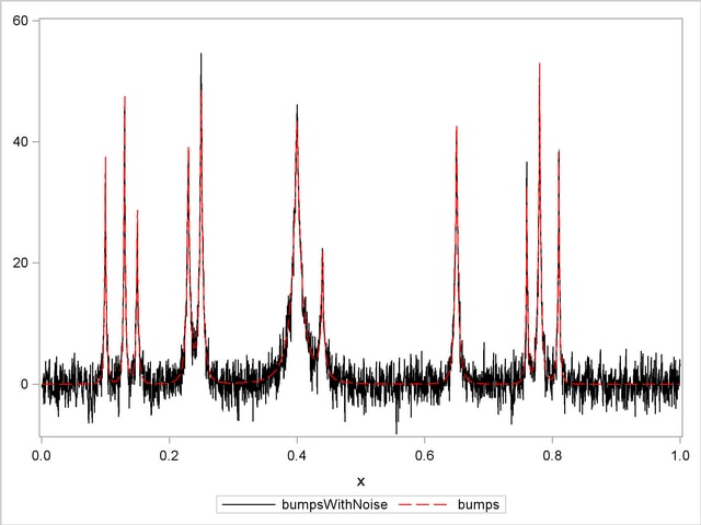
The following statements use the SGPLOT procedure to produce the plot in Output 42.3.1. The plot shows the bumps function superimposed on the function with added noise.
   proc sgplot data=DoJoBumps;
     yaxis display=(nolabel);
     series  x=x y=bumpsWithNoise/lineattrs=(color=black);
     series  x=x y=bumps/lineattrs=(color=red);
   run;
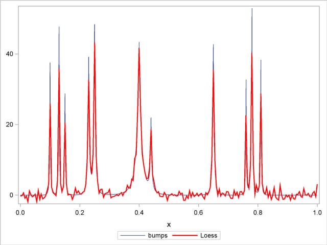
Suppose you want to smooth the noisy data to recover the underlying function. This problem is studied by Sarle (2001), who shows how neural nets can be used to perform the smoothing. The following statements use the LOESS statement in the SGPLOT procedure to show a loess fit superimposed on the noisy data (Output 42.3.2). (See Chapter 50, The LOESS Procedure, for information about the loess method.)
   proc sgplot data=DoJoBumps;
      yaxis display=(nolabel);
      series x=x y=bumps;
      loess  x=x y=bumpsWithNoise / lineattrs=(color=red) nomarkers;
   run;
The algorithm selects a smoothing parameter that is small enough to enable bumps to be resolved. Because there is a single smoothing parameter that controls the number of points for all local fits, the loess method undersmooths the function in the intervals between the bumps.
Another approach to doing nonparametric fitting is to approximate the unknown underlying function as a linear combination of a set of basis functions. Once you specify the basis functions, then you can use least squares regression to obtain the coefficients of the linear combination. A problem with this approach is that for most data, you do not know a priori what set of basis functions to use. You need to supply a sufficiently rich set to enable the features in the data to be approximated. However, if you use too rich a set of functions, then this approach yields a fit that undersmooths the data and captures spurious features in the noise.
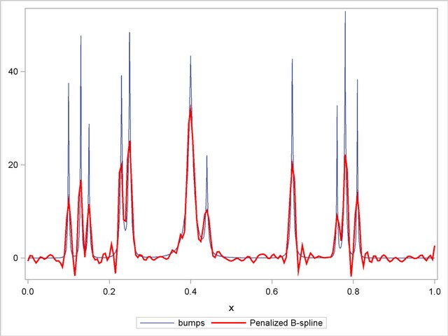
The penalized B-spline method (Eilers and Marx 1996) uses a basis of B-splines (see the section Constructed Effects and the EFFECT Statement of Chapter 18, Shared Concepts and Topics ) corresponding to a large number of equally spaced knots as the set of approximating functions. To control the potential overfitting, their algorithm modifies the least squares objective function to include a penalty term that grows with the complexity of the fit.
The following statements use the PBSPLINE statement in the SGPLOT procedure to show a penalized B-spline fit superimposed on the noisy data (Output 42.3.3). See Chapter 90, The TRANSREG Procedure, for details about the implementation of the penalized B-spline method.
   proc sgplot data=DoJoBumps;
      yaxis display=(nolabel);
      series    x=x y=bumps;
      pbspline  x=x y=bumpsWithNoise /
                  lineattrs=(color=red) nomarkers;
   run;
As in the case of loess fitting, you see undersmoothing in the intervals between the bumps because there is only a single smoothing parameter that controls the overall smoothness of the fit.
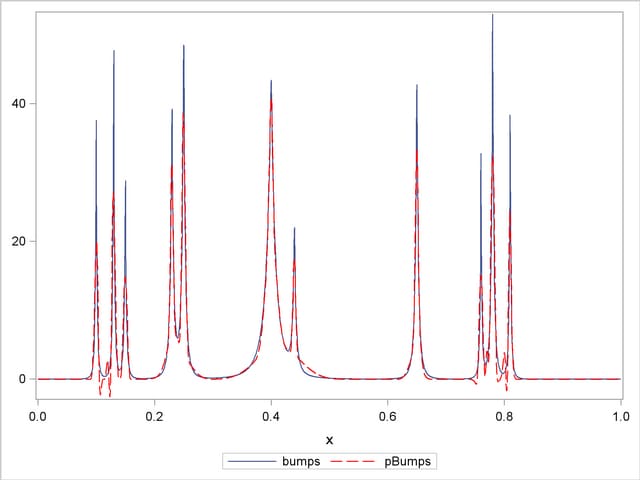
An alternative to using a smoothness penalty to control the overfitting is to use variable selection to obtain an appropriate subset of the basis functions. In order to be able to represent features in the data that occur at multiple scales, it is useful to select from B-spline functions defined on just a few knots to capture large scale features of the data as well as B-spline functions defined on many knots to capture fine details of the data. The following statements show how you can use PROC GLMSELECT to implement this strategy:
   proc glmselect data=dojoBumps;
      effect spl = spline(x / knotmethod=multiscale(endscale=8)
                                split details);
      model bumpsWithNoise=spl;
      output out=out1 p=pBumps;
   run;

   proc sgplot data=out1;
      yaxis display=(nolabel);
      series    x=x y=bumps;
      series    x=x y=pBumps / lineattrs=(color=red);
   run;
The KNOTMETHOD=MULTISCALE suboption of the EFFECT spl = SPLINE statement provides a convenient way to generate B-spline basis functions at multiple scales. The ENDSCALE=8 option requests that the finest scale use B-splines defined on  equally spaced knots in the interval
  . Because the cubic B-splines are nonzero over five adjacent knots, at the finest scale, the support of each B-spline basis function is an interval of length about
  (5/256), enabling the bumps in the underlying data to be resolved. The default value is ENDSCALE=7. At this scale you will still be able to capture the bumps, but with less sharp resolution. For these data, using a value of ENDSCALE= greater than eight provides unneeded resolution, making it more likely that basis functions that fit spurious features in the noise are selected.
Output 42.3.4 shows the model information table. Since no options are specified in the MODEL statement, PROC GLMSELECT uses the stepwise method with selection and stopping based on the SBC criterion.
| Data Set | WORK.DOJOBUMPS |
|---|---|
| Dependent Variable | bumpsWithNoise |
| Selection Method | Stepwise |
| Select Criterion | SBC |
| Stop Criterion | SBC |
| Effect Hierarchy Enforced | None |
The DETAILS suboption in the EFFECT statement requests the display of spline knots and spline basis tables. These tables contain information about knots and basis functions at all scales. The results for scale four are shown in Output 42.3.5 and Output 42.3.6.
| Knots for Spline Effect spl | ||||
|---|---|---|---|---|
| Knot Number | Scale | Scale Knot Number | Boundary | x |
| 40 | 4 | 1 | * | -0.11735 |
| 41 | 4 | 2 | * | -0.05855 |
| 42 | 4 | 3 | * | 0.00024414 |
| 43 | 4 | 4 | 0.05904 | |
| 44 | 4 | 5 | 0.11783 | |
| 45 | 4 | 6 | 0.17663 | |
| 46 | 4 | 7 | 0.23542 | |
| 47 | 4 | 8 | 0.29422 | |
| 48 | 4 | 9 | 0.35301 | |
| 49 | 4 | 10 | 0.41181 | |
| 50 | 4 | 11 | 0.47060 | |
| 51 | 4 | 12 | 0.52940 | |
| 52 | 4 | 13 | 0.58819 | |
| 53 | 4 | 14 | 0.64699 | |
| 54 | 4 | 15 | 0.70578 | |
| 55 | 4 | 16 | 0.76458 | |
| 56 | 4 | 17 | 0.82337 | |
| 57 | 4 | 18 | 0.88217 | |
| 58 | 4 | 19 | 0.94096 | |
| 59 | 4 | 20 | * | 0.99976 |
| 60 | 4 | 21 | * | 1.05855 |
| 61 | 4 | 22 | * | 1.11735 |
| Basis Details for Spline Effect spl | |||||
|---|---|---|---|---|---|
| Column | Scale | Scale Column | Support | Support Knots | |
| 32 | 4 | 1 | -0.11735 | 0.05904 | 1-4 |
| 33 | 4 | 2 | -0.11735 | 0.11783 | 1-5 |
| 34 | 4 | 3 | -0.05855 | 0.17663 | 2-6 |
| 35 | 4 | 4 | 0.00024414 | 0.23542 | 3-7 |
| 36 | 4 | 5 | 0.05904 | 0.29422 | 4-8 |
| 37 | 4 | 6 | 0.11783 | 0.35301 | 5-9 |
| 38 | 4 | 7 | 0.17663 | 0.41181 | 6-10 |
| 39 | 4 | 8 | 0.23542 | 0.47060 | 7-11 |
| 40 | 4 | 9 | 0.29422 | 0.52940 | 8-12 |
| 41 | 4 | 10 | 0.35301 | 0.58819 | 9-13 |
| 42 | 4 | 11 | 0.41181 | 0.64699 | 10-14 |
| 43 | 4 | 12 | 0.47060 | 0.70578 | 11-15 |
| 44 | 4 | 13 | 0.52940 | 0.76458 | 12-16 |
| 45 | 4 | 14 | 0.58819 | 0.82337 | 13-17 |
| 46 | 4 | 15 | 0.64699 | 0.88217 | 14-18 |
| 47 | 4 | 16 | 0.70578 | 0.94096 | 15-19 |
| 48 | 4 | 17 | 0.76458 | 0.99976 | 16-20 |
| 49 | 4 | 18 | 0.82337 | 1.05855 | 17-21 |
| 50 | 4 | 19 | 0.88217 | 1.11735 | 18-22 |
| 51 | 4 | 20 | 0.94096 | 1.11735 | 19-22 |
The "Dimensions" table in Output 42.3.7 shows that at each step of the selection process, 548 effects are considered as candidates for entry or removal. Note that although the MODEL statement specifies a single constructed effect spl, the SPLIT suboption causes each of the parameters in this constructed effect to be treated as an individual effect.
Output 42.3.8 shows the parameter estimates for the selected model. You can see that the selected model contains 31 B-spline basis functions and that all the selected B-spline basis functions are from scales four though eight. For example, the first basis function listed in the parameter estimates table is spl_S4:9—the 9th B-spline function at scale 4. You see from Output 42.3.6 that this function is nonzero on the interval  .
.
| Parameter Estimates | ||||
|---|---|---|---|---|
| Parameter | DF | Estimate | Standard Error | t Value |
| Intercept | 1 | -0.009039 | 0.077412 | -0.12 |
| spl_S4:9 | 1 | 7.070207 | 0.586990 | 12.04 |
| spl_S5:10 | 1 | 5.323121 | 1.199824 | 4.44 |
| spl_S6:17 | 1 | 5.222808 | 1.728910 | 3.02 |
| spl_S6:28 | 1 | 24.562103 | 1.490639 | 16.48 |
| spl_S6:44 | 1 | 4.930829 | 1.243552 | 3.97 |
| spl_S6:52 | 1 | -7.046308 | 2.487700 | -2.83 |
| spl_S7:86 | 1 | 9.592742 | 2.626471 | 3.65 |
| spl_S7:106 | 1 | 16.268550 | 3.334015 | 4.88 |
| spl_S8:27 | 1 | 10.626586 | 1.752152 | 6.06 |
| spl_S8:28 | 1 | 27.882444 | 2.004520 | 13.91 |
| spl_S8:29 | 1 | -6.129939 | 1.752151 | -3.50 |
| spl_S8:33 | 1 | 5.855648 | 1.766912 | 3.31 |
| spl_S8:34 | 1 | -11.782303 | 2.092484 | -5.63 |
| spl_S8:35 | 1 | 38.705178 | 2.092486 | 18.50 |
| spl_S8:36 | 1 | 13.823256 | 1.766916 | 7.82 |
| spl_S8:40 | 1 | 15.975124 | 1.691679 | 9.44 |
| spl_S8:41 | 1 | 14.898716 | 1.691679 | 8.81 |
| spl_S8:61 | 1 | 37.441965 | 2.084375 | 17.96 |
| spl_S8:66 | 1 | 47.484506 | 1.883409 | 25.21 |
| spl_S8:67 | 1 | 16.811502 | 1.910358 | 8.80 |
| spl_S8:104 | 1 | 11.098484 | 1.958676 | 5.67 |
| spl_S8:105 | 1 | 26.704556 | 2.042735 | 13.07 |
| spl_S8:115 | 1 | 21.102920 | 1.576185 | 13.39 |
| spl_S8:169 | 1 | 36.572294 | 2.914521 | 12.55 |
| spl_S8:197 | 1 | 20.869716 | 1.882529 | 11.09 |
| spl_S8:198 | 1 | 16.210987 | 2.693183 | 6.02 |
| spl_S8:200 | 1 | 13.113942 | 3.458187 | 3.79 |
| spl_S8:202 | 1 | 38.463549 | 2.462314 | 15.62 |
| spl_S8:203 | 1 | 34.164644 | 1.757908 | 19.43 |
| spl_S8:209 | 1 | -22.645471 | 3.598587 | -6.29 |
| spl_S8:210 | 1 | 29.024741 | 2.557567 | 11.35 |
The OUTPUT statement captures the predicted values in a data set named out1, and Output 42.3.9 shows a fit plot produced by PROC SGPLOT.
Copyright © 2009 by SAS Institute Inc., Cary, NC, USA. All rights reserved.