If there are exogenous manifest variables in the linear structural equation model, then there is a one-to-one relationship between the given covariances and corresponding estimates in the central model matrix ( or ). In general, using exogenous manifest variables reduces the degrees of freedom since the corresponding sample correlations or covariances are not part of the exogenous information provided for the parameter estimation. See the section Counting the Degrees of Freedom for more information.

If you specify a RAM or LINEQS model statement, or if such a model is recognized in an INRAM= data set, those elements in the central model matrices that correspond to the exogenous manifest variables are reset to the sample values after computing covariances or correlations within the current BY group.

The COSAN statement does not automatically set the covariances in the central model matrices that correspond to manifest exogenous variables.

You can use the output of the predetermined values in the predicted model matrix (PREDET option) that correspond to manifest exogenous variables to see which of the manifest variables are exogenous variables and to help you set the corresponding locations of the central model matrices with their covariances.

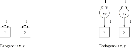
The following two examples show how different the results of PROC CALIS can be if manifest variables are considered as either endogenous or exogenous variables. (See Figure 25.5.) In both examples, a correlation matrix is tested against an identity model matrix ; that is, no parameter is estimated. The following three runs of the first example (specified by the COSAN, LINEQS, and RAM statements) consider the two variables and as endogenous variables:

   title2 'Data: FULLER (1987, p.18)';
   data corn;
      input y x;
      datalines;
    86  70
   115  97
    90  53
    86  64
   110  95
    91  64
    99  50
    96  70
    99  94
   104  69
    96  51
   ;

   title3 'Endogenous Y and X';
   proc calis data=corn;
      cosan corr(2,ide);
   run;
   proc calis data=corn;
      lineqs
             y=ey,
             x=ex;
      std    ey ex=2 * 1;
   run;
   proc calis data=corn;
      ram
          1  1  3  1.,
          1  2  4  1.,
          2  3  3  1.,
          2  4  4  1.;
   run;

The following two runs of the second example (specified by the LINEQS and RAM statements) consider and as exogenous variables:

   title3 'Exogenous Y and X';
   proc calis data=corn;
      std y x=2 * 1;
   run;
   proc calis data=corn;
      ram
          2  1  1  1.,
          2  2  2  1.;
   run;

Figure 25.5 Exogenous and Endogenous Variables

The LINEQS and the RAM model statements set the covariances (correlations) of exogenous manifest variables in the estimated model matrix and automatically reduce the degrees of freedom.