| The CALIS Procedure |
| Assessment of Fit |
This section contains a collection of formulas used in computing indices to assess the goodness of fit by PROC CALIS. The following notation is used:
 for the sample size
  for the number of manifest variables
  for the number of parameters to estimate
 for the degrees of freedom
  for the vector of optimal parameter estimates
  for the
  input COV, CORR, UCOV, or UCORR matrix
 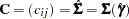 for the predicted model matrix
  for the weight matrix (
 for ULS,
  for default GLS, and
  for ML estimates)
  for the
  asymptotic covariance matrix of sample covariances
  for the cumulative distribution function of the noncentral chi-squared distribution with noncentrality parameter
The following notation is for indices that support testing nested models by a  difference test:
 for the function value of the independence model
  for the degrees of freedom of the independence model
  for the function value of the fitted model
  for the degrees of freedom of the fitted model
The degrees of freedom  and the number of parameters are adjusted automatically when there are active constraints in the analysis. The computation of many fit statistics and indices are affected. You can turn off the automatic adjustment by using the NOADJDF option. See the section Counting the Degrees of Freedom for more information.
Residuals
PROC CALIS computes four types of residuals and writes them to the OUTSTAT= data set.
Raw Residuals

The raw residuals are displayed whenever the PALL, PRINT, or RESIDUAL option is specified.
Variance Standardized Residuals
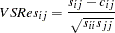
The variance standardized residuals are displayed when you specify the following:
the PALL, PRINT, or RESIDUAL option and METHOD=NONE, METHOD=ULS, or METHOD=DWLS
RESIDUAL=VARSTAND
The variance standardized residuals are equal to those computed by the EQS 3 program (Bentler 1989).
Asymptotically Standardized Residuals

The matrix
 is the
  Jacobian matrix
  , and
, and  is the
  asymptotic covariance matrix of parameter estimates (the inverse of the information matrix). Asymptotically standardized residuals are displayed when one of the following conditions is met:
 The PALL, PRINT, or RESIDUAL option is specified, and METHOD=ML, METHOD=GLS, or METHOD=WLS, and the expensive information and Jacobian matrices are computed for some other reason.
RESIDUAL= ASYSTAND is specified.
The asymptotically standardized residuals are equal to those computed by the LISREL 7 program (Jöreskog and Sörbom 1988) except for the denominator
 in the definition of matrix .
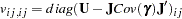
 Normalized Residuals
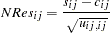
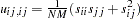
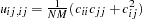
where the diagonal elements
 of the asymptotic covariance matrix of sample covariances are defined for the following methods.
 GLS as
ML as
WLS as

Normalized residuals are displayed when one of the following conditions is met:
The PALL, PRINT, or RESIDUAL option is specified, and METHOD=ML, METHOD=GLS, or METHOD=WLS, and the expensive information and Jacobian matrices are not computed for some other reason.
RESIDUAL=NORM is specified.
The normalized residuals are equal to those computed by the LISREL VI program (Jöreskog and Sörbom 1985) except for the definition of the denominator
in matrix .
For estimation methods that are not BGLS estimation methods (Browne 1982, 1984), such as METHOD=NONE, METHOD=ULS, or METHOD=DWLS, the assumption of an asymptotic covariance matrix of sample covariances does not seem to be appropriate. In this case, the normalized residuals should be replaced by the more relaxed variance standardized residuals. Computation of asymptotically standardized residuals requires computing the Jacobian and information matrices. This is computationally very expensive and is done only if the Jacobian matrix has to be computed for some other reason—that is, if at least one of the following items is true:
The default, PRINT, or PALL displayed output is requested, and neither the NOMOD nor NOSTDERR option is specified.
Either the MODIFICATION (included in PALL), PCOVES, or STDERR (included in default, PRINT, and PALL output) option is requested or RESIDUAL=ASYSTAND is specified.
The LEVMAR or NEWRAP optimization technique is used.
An OUTRAM= data set is specified without using the NOSTDERR option.
An OUTEST= data set is specified without using the NOSTDERR option.
Since normalized residuals use an overestimate of the asymptotic covariance matrix of residuals (the diagonal of ), the normalized residuals cannot be larger than the asymptotically standardized residuals (which use the diagonal of  ).
).
Together with the residual matrices, the values of the average residual, the average off-diagonal residual, and the rank order of the largest values are displayed. The distribution of the normalized and standardized residuals is displayed also.
Goodness of Fit Indices Based on Residuals
The following items are computed for all five kinds of estimation: ULS, GLS, ML, WLS, and DWLS. All these indices are written to the OUTRAM= data set. The goodness of fit (GFI), adjusted goodness of fit (AGFI), and root mean square residual (RMR) are computed as in the LISREL VI program of Jöreskog and Sörbom (1985).
Goodness of Fit Index
The goodness of fit index for the ULS, GLS, and ML estimation methods is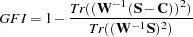
but for WLS and DWLS estimation, it is
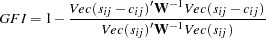
where
 for DWLS estimation, and
  denotes the vector of the
  elements of the lower triangle of the symmetric matrix
  . For a constant weight matrix , the goodness of fit index is 1 minus the ratio of the minimum function value and the function value before any model has been fitted. The GFI should be between 0 and 1. The data probably do not fit the model if the GFI is negative or much larger than 1.
 Adjusted Goodness of Fit Index
The AGFI is the GFI adjusted for the degrees of freedom of the model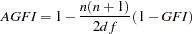
The AGFI corresponds to the GFI in replacing the total sum of squares by the mean sum of squares.
Caution:
Large
and small can result in a negative AGFI. For example, GFI ,
,  , and
, and  result in an AGFI of
  .
. AGFI is not defined for a saturated model, due to division by
 .
. AGFI is not sensitive to losses in
.
The AGFI should be between 0 and 1. The data probably do not fit the model if the AGFI is negative or much larger than 1. For more information, refer to Mulaik et al. (1989).
Root Mean Square Residual
The RMR is the root of the mean of the squared residuals: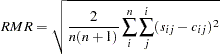
Standardized Root Mean Square Residual
The SRMR is the root of the mean of the squared standardized residuals: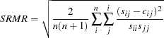
Parsimonious Goodness of Fit Index
The PGFI (Mulaik et al. 1989) is a modification of the GFI that takes the parsimony of the model into account: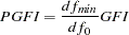
The PGFI uses the same parsimonious factor as the parsimonious normed Bentler-Bonett index (James, Mulaik, and Brett 1982).
Goodness of Fit Indices Based on the 
The following items are transformations of the overall value and in general depend on the sample size N. These indices are not computed for ULS or DWLS estimates.
Uncorrected
The overall measure is the optimum function value  multiplied by
  if a CORR or COV matrix is analyzed, or multiplied by if a UCORR or UCOV matrix is analyzed. This gives the likelihood ratio test statistic for the null hypothesis that the predicted matrix
  has the specified model structure against the alternative that is unconstrained. The test is valid only if the observations are independent and identically distributed, the analysis is based on the nonstandardized sample covariance matrix
  , and the sample size is sufficiently large (Browne 1982; Bollen 1989b; Jöreskog and Sörbom 1985). For ML and GLS estimates, the variables must also have an approximately multivariate normal distribution. The notation Prob>Chi**2 means "the probability under the null hypothesis of obtaining a greater statistic than that observed."
where
is the function value at the minimum.  Value of the Independence Model
The value of the independence model 
and the corresponding degrees of freedom
can be used (in large samples) to evaluate the gain of explanation by fitting the specific model (Bentler 1989). RMSEA Index (Steiger and Lind 1980)
The Steiger and Lind (1980) root mean squared error approximation (RMSEA) coefficient is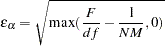
The lower and upper limits of the confidence interval are computed using the cumulative distribution function of the noncentral chi-squared distribution
 , with
  ,
,  satisfying
 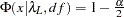 , and
, and  satisfying
 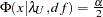 :
: 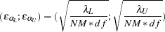
Refer to Browne and Du Toit (1992) for more details. The size of the confidence interval is defined by the option ALPHARMS=
 ,
,  . The default is
  , which corresponds to the 90% confidence interval for the RMSEA.
 Probability for Test of Close Fit (Browne and Cudeck 1993)
The traditional exact test hypothesis  is replaced by the null hypothesis of close fit
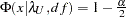
  and the exceedance probability
  is computed as
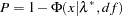
where
and 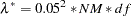 . The null hypothesis of close fit is rejected if is smaller than a prespecified level (for example,
  ).
). Expected Cross Validation Index (Browne and Cudeck 1993)
For GLS and WLS, the estimator of the ECVI is linearly related to AIC:
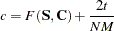
For ML estimation,
 is used.
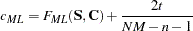
The confidence interval
 for is computed using the cumulative distribution function of the noncentral chi-squared distribution,
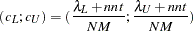
with
 ,
,  ,
,  , and
, and  . The confidence interval
  for is
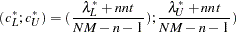
where
,  ,
,  and
and  . Refer to Browne and Cudeck (1993) for details. The size of the confidence interval is defined by the option ALPHAECV=, . The default is , which corresponds to the 90% confidence interval for the ECVI.
 Comparative Fit Index (Bentler 1989)
Adjusted
Value (Browne 1982)
If the variables are-variate elliptic rather than normal and have significant amounts of multivariate kurtosis (leptokurtic or platykurtic), the value can be adjusted to 
where
 is the multivariate relative kurtosis coefficient.
 Normal Theory Reweighted LS
Value
This index is displayed only if METHOD=ML. Instead of the function value , the reweighted goodness of fit function
  is used,
where
is the value of the function at the minimum. Akaike’s Information Criterion (AIC) (Akaike 1974; Akaike 1987)
This is a criterion for selecting the best model among a number of candidate models. The model that yields the smallest value of AIC is considered the best.
Consistent Akaike’s Information Criterion (CAIC) (Bozdogan 1987)
This is another criterion, similar to AIC, for selecting the best model among alternatives. The model that yields the smallest value of CAIC is considered the best. CAIC is preferred by some people to AIC or the test. 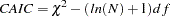
Schwarz’s Bayesian Criterion (SBC) (Schwarz 1978; Sclove 1987)
This is another criterion, similar to AIC, for selecting the best model. The model that yields the smallest value of SBC is considered the best. SBC is preferred by some people to AIC or the test. 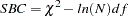
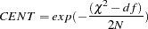
McDonald’s Measure of Centrality (McDonald 1989)
Parsimonious Normed Fit Index (James, Mulaik, and Brett 1982)
The PNFI is a modification of Bentler-Bonett’s normed fit index that takes parsimony of the model into account,
The PNFI uses the same parsimonious factor as the parsimonious GFI of Mulaik et al. (1989).
Z-Test (Wilson and Hilferty 1931)
The Z-test of Wilson and Hilferty assumes an-variate normal distribution: 
Refer to McArdle (1988) and Bishop, Fienberg, and Holland (1977, p. 527) for an application of the Z-test.
Nonnormed Coefficient (Bentler and Bonett 1980)
Refer to Tucker and Lewis (1973) for details.
Normed Coefficient (Bentler and Bonett 1980)

Mulaik et al. (1989) recommend the parsimonious weighted form PNFI.
Normed Index
 (Bollen 1986)
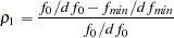
 is always less than or equal to
  ;
;  is unlikely in practice. Refer to the discussion in Bollen (1989a) for details.
 Nonnormed Index
 (Bollen 1989a)
is a modification of Bentler and Bonett’s
 that uses and "lessens the dependence" on . Refer to the discussion in Bollen (1989b).
  is identical to Mulaik et al.’s (1989) IFI2 index.
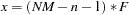
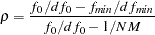
 Critical N Index (Hoelter 1983)

where
 is the critical chi-square value for the given degrees of freedom and probability
  , and is the value of the estimation criterion (minimization function). Refer to Bollen (1989b, p. 277) for details. Hoelter (1983) suggests that CN should be at least 200; however, Bollen (1989b) notes that the CN value might lead to an overly pessimistic assessment of fit for small samples.
Squared Multiple Correlation
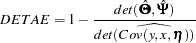
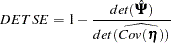
The following are measures of the squared multiple correlation for manifest and endogenous variables and are computed for all five estimation methods: ULS, GLS, ML, WLS, and DWLS. These coefficients are computed as in the LISREL VI program of Jöreskog and Sörbom (1985). The DETAE, DETSE, and DETMV determination coefficients are intended to be global means of the squared multiple correlations for different subsets of model equations and variables. These coefficients are displayed only when you specify the PDETERM option with a RAM or LINEQS model.
 Values Corresponding to Endogenous Variables
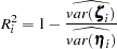
Total Determination of All Equations
Total Determination of the Structural Equations
Total Determination of the Manifest Variables
Caution:In the LISREL program, the structural equations are defined by specifying the BETA matrix. In PROC CALIS, a structural equation has a dependent left-hand-side variable that appears at least once on the right-hand side of another equation, or the equation has at least one right-hand-side variable that is the left-hand-side variable of another equation. Therefore, PROC CALIS sometimes identifies more equations as structural equations than the LISREL program does.
Copyright © 2009 by SAS Institute Inc., Cary, NC, USA. All rights reserved.