The HPPRINCOMP Procedure

Getting Started: HPPRINCOMP Procedure

The following data provide crime rates per 100,000 people in seven categories for each of the 50 US states in 1977:

title 'Crime Rates per 100,000 Population by State';

data Crime;
   input State $1-15 Murder Rape Robbery Assault
         Burglary Larceny Auto_Theft;
   datalines;
Alabama        14.2 25.2  96.8 278.3 1135.5 1881.9 280.7
Alaska         10.8 51.6  96.8 284.0 1331.7 3369.8 753.3
Arizona         9.5 34.2 138.2 312.3 2346.1 4467.4 439.5
Arkansas        8.8 27.6  83.2 203.4  972.6 1862.1 183.4
California     11.5 49.4 287.0 358.0 2139.4 3499.8 663.5
Colorado        6.3 42.0 170.7 292.9 1935.2 3903.2 477.1
Connecticut     4.2 16.8 129.5 131.8 1346.0 2620.7 593.2
Delaware        6.0 24.9 157.0 194.2 1682.6 3678.4 467.0
Florida        10.2 39.6 187.9 449.1 1859.9 3840.5 351.4
Georgia        11.7 31.1 140.5 256.5 1351.1 2170.2 297.9
Hawaii          7.2 25.5 128.0  64.1 1911.5 3920.4 489.4
Idaho           5.5 19.4  39.6 172.5 1050.8 2599.6 237.6
Illinois        9.9 21.8 211.3 209.0 1085.0 2828.5 528.6
Indiana         7.4 26.5 123.2 153.5 1086.2 2498.7 377.4
Iowa            2.3 10.6  41.2  89.8  812.5 2685.1 219.9
Kansas          6.6 22.0 100.7 180.5 1270.4 2739.3 244.3
Kentucky       10.1 19.1  81.1 123.3  872.2 1662.1 245.4
Louisiana      15.5 30.9 142.9 335.5 1165.5 2469.9 337.7
Maine           2.4 13.5  38.7 170.0 1253.1 2350.7 246.9
Maryland        8.0 34.8 292.1 358.9 1400.0 3177.7 428.5
Massachusetts   3.1 20.8 169.1 231.6 1532.2 2311.3 1140.1
Michigan        9.3 38.9 261.9 274.6 1522.7 3159.0 545.5
Minnesota       2.7 19.5  85.9  85.8 1134.7 2559.3 343.1
Mississippi    14.3 19.6  65.7 189.1  915.6 1239.9 144.4
Missouri        9.6 28.3 189.0 233.5 1318.3 2424.2 378.4
Montana         5.4 16.7  39.2 156.8  804.9 2773.2 309.2
Nebraska        3.9 18.1  64.7 112.7  760.0 2316.1 249.1
Nevada         15.8 49.1 323.1 355.0 2453.1 4212.6 559.2
New Hampshire   3.2 10.7  23.2  76.0 1041.7 2343.9 293.4
New Jersey      5.6 21.0 180.4 185.1 1435.8 2774.5 511.5
New Mexico      8.8 39.1 109.6 343.4 1418.7 3008.6 259.5
New York       10.7 29.4 472.6 319.1 1728.0 2782.0 745.8
North Carolina 10.6 17.0  61.3 318.3 1154.1 2037.8 192.1
North Dakota    0.9  9.0  13.3  43.8  446.1 1843.0 144.7
Ohio            7.8 27.3 190.5 181.1 1216.0 2696.8 400.4
Oklahoma        8.6 29.2  73.8 205.0 1288.2 2228.1 326.8
Oregon          4.9 39.9 124.1 286.9 1636.4 3506.1 388.9
Pennsylvania    5.6 19.0 130.3 128.0  877.5 1624.1 333.2
Rhode Island    3.6 10.5  86.5 201.0 1489.5 2844.1 791.4
South Carolina 11.9 33.0 105.9 485.3 1613.6 2342.4 245.1
South Dakota    2.0 13.5  17.9 155.7  570.5 1704.4 147.5
Tennessee      10.1 29.7 145.8 203.9 1259.7 1776.5 314.0
Texas          13.3 33.8 152.4 208.2 1603.1 2988.7 397.6
Utah            3.5 20.3  68.8 147.3 1171.6 3004.6 334.5
Vermont         1.4 15.9  30.8 101.2 1348.2 2201.0 265.2
Virginia        9.0 23.3  92.1 165.7  986.2 2521.2 226.7
Washington      4.3 39.6 106.2 224.8 1605.6 3386.9 360.3
West Virginia   6.0 13.2  42.2    .  597.4 1341.7 163.3
Wisconsin       2.8 12.9  52.2  63.7  846.9 2614.2 220.7
Wyoming          .  21.9  39.7 173.9  811.6 2772.2 282.0
;

The following statements invoke the HPPRINCOMP procedure, which requests a principal component analysis of the data and produces Figure 13.1 through Figure 13.4:

proc hpprincomp data=Crime;
run;

Figure 13.1 displays the "Performance Information," "Data Access Information," "Model Information," "Number of Observations," "Number of Variables," and "Simple Statistics" tables.

The "Performance Information" table shows the procedure executes in single-machine mode—that is, the data reside and the computation is performed on the machine where the SAS session executes. This run of the HPPRINCOMP procedure took place on a multicore machine with four CPUs; one computational thread was spawned per CPU.

The "Data Access Information" table shows that the input data set is accessed with the V9 (base) engine on the client machine where the MVA SAS session executes.

The "Model Information" table identifies the data source and shows that the principal component extraction method is eigenvalue decomposition, which is the default.

The "Number of Observations" table shows that of the 50 observations in the input data, only 48 observations are used in the analysis because some observations have incomplete data.

The "Number of Variables" table indicates that there are seven variables to be analyzed and seven principal components to be computed. By default, if the VAR statement is omitted, all numeric variables that are not listed in other statements are used in the analysis.

The "Simple Statistics" table displays the mean and standard deviation of the analysis variables.

Figure 13.1: Performance Information and Simple Statistics

Crime Rates per 100,000 Population by State

The HPPRINCOMP Procedure

Performance Information
Execution Mode	Single-Machine
Number of Threads	4

Data Access Information
Data	Engine	Role	Path
WORK.CRIME	V9	Input	On Client

Model Information
Data Source	WORK.CRIME
Component Extraction Method	Eigenvalue Decomposition

Number of Observations Read	50
Number of Observations Used	48

Number of Variables	7
Number of Principal Components	7

Simple Statistics
Variable	Mean	Standard Deviation
Murder	7.51667	3.93059
Rape	26.07500	10.81304
Robbery	127.55625	88.49374
Assault	214.58750	100.64360
Burglary	1316.37917	423.31261
Larceny	2696.88542	714.75023
Auto_Theft	383.97917	194.37033

Figure 13.2 displays the "Correlation Matrix" table. By default, the PROC HPPRINCOMP statement requests that principal components be computed from the correlation matrix, so the total variance is equal to the number of variables, 7.

Figure 13.2: Correlation Matrix Table

Correlation Matrix
Variable	Murder	Rape	Robbery	Assault	Burglary	Larceny	Auto_Theft
Murder	1.0000	0.6000	0.4768	0.6485	0.3778	0.0925	0.0555
Rape	0.6000	1.0000	0.5817	0.7316	0.7038	0.6009	0.3282
Robbery	0.4768	0.5817	1.0000	0.5452	0.6200	0.4371	0.5787
Assault	0.6485	0.7316	0.5452	1.0000	0.6082	0.3791	0.2520
Burglary	0.3778	0.7038	0.6200	0.6082	1.0000	0.7932	0.5390
Larceny	0.0925	0.6009	0.4371	0.3791	0.7932	1.0000	0.4246
Auto_Theft	0.0555	0.3282	0.5787	0.2520	0.5390	0.4246	1.0000

Figure 13.3 displays the "Eigenvalues" table. The first principal component accounts for about 57.8% of the total variance, the second principal component accounts for about 18.1%, and the third principal component accounts for about 10.7%. Note that the eigenvalues sum to the total variance.

The eigenvalues indicate that two or three components provide a good summary of the data: two components account for 76% of the total variance, and three components account for 87%. Subsequent components account for less than 5% each.

Figure 13.3: Eigenvalues Table

Eigenvalues of the Correlation Matrix
	Eigenvalue	Difference	Proportion	Cumulative
1	4.045824	2.781795	0.5780	0.5780
2	1.264030	0.516529	0.1806	0.7586
3	0.747500	0.421175	0.1068	0.8653
4	0.326325	0.061119	0.0466	0.9120
5	0.265207	0.036843	0.0379	0.9498
6	0.228364	0.105613	0.0326	0.9825
7	0.122750		0.0175	1.0000

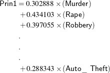
Figure 13.4 displays the "Eigenvectors" table. From the eigenvectors matrix, you can represent the first principal component, Prin1, as a linear combination of the original variables:

$\begin{align*} \mr{\Variable{Prin1}} & = 0.302888 \times (\mr{\Variable{Murder}})\\ & \mr{\ } + 0.434103 \times (\mr{\Variable{Rape}}) \\ & \mr{\ } + 0.397055 \times (\mr{\Variable{Robbery}}) \\ & \mr{\ } . \\ & \mr{\ } . \\ & \mr{\ } . \\ & \mr{\ } + 0.288343 \times (\mr{\Variable{Auto\_ Theft}}) \end{align*}$

Similarly, the second principal component, Prin2, is

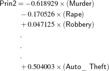
$\begin{align*} \mr{\Variable{Prin2}} & = - 0.618929 \times (\mr{\Variable{Murder}})\\ & \mr{~ ~ } - 0.170526 \times (\mr{\Variable{Rape}})\\ & \mr{~ ~ } + 0.047125 \times (\mr{\Variable{Robbery}}) \\ & \mr{~ ~ } . \\ & \mr{~ ~ } . \\ & \mr{~ ~ } . \\ & \mr{~ ~ } + 0.504003 \times (\mr{\Variable{Auto\_ Theft}}) \end{align*}$

where the variables are standardized.

Figure 13.4: Eigenvectors Table

Eigenvectors
Variable	Prin1	Prin2	Prin3	Prin4	Prin5	Prin6	Prin7
Murder	0.30289	-0.61893	0.17353	-0.23308	0.54896	0.26371	0.26428
Rape	0.43410	-0.17053	-0.23539	0.06540	0.18075	-0.78232	-0.27946
Robbery	0.39705	0.04713	0.49208	-0.57470	-0.50808	-0.09452	-0.02497
Assault	0.39622	-0.35142	-0.05343	0.61743	-0.51525	0.17395	0.19921
Burglary	0.44164	0.20861	-0.22454	-0.02750	0.11273	0.52340	-0.65085
Larceny	0.35634	0.40570	-0.53681	-0.23231	0.02172	0.04085	0.60346
Auto_Theft	0.28834	0.50400	0.57524	0.41853	0.35939	-0.06024	0.15487

The first component is a measure of the overall crime rate, because the first eigenvector shows approximately equal loadings on all variables. The second eigenvector has high positive loadings on the variables Auto_Theft and Larceny and high negative loadings on the variables Murder and Assault. There is also a small positive loading on the variable Burglary and a small negative loading on the variable Rape. This component seems to measure the preponderance of property crime compared to violent crime. The interpretation of the third component is not obvious.