The HPGENSELECT Procedure
-
Overview

- Getting Started
-
Syntax
-
DetailsMissing ValuesExponential Family DistributionsResponse DistributionsResponse Probability Distribution FunctionsLog-Likelihood FunctionsThe LASSO Method of Model SelectionUsing Validation and Test DataComputational Method: MultithreadingChoosing an Optimization AlgorithmDisplayed OutputODS Table Names
-
Examples
- References
Response Probability Distribution Functions
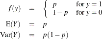
Binary Distribution
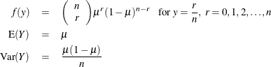
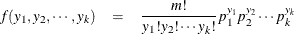
Binomial Distribution
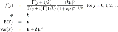
Gamma Distribution
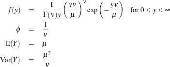
For the gamma distribution,  is the estimated dispersion parameter that is displayed in the output. The parameter
  is also sometimes called the gamma index parameter.
Inverse Gaussian Distribution
![\begin{eqnarray*} f(y) & = & \frac{1}{\sqrt {2\pi y^3} \sigma } \exp \left[ -\frac{1}{2y} \left( \frac{y-\mu }{\mu \sigma } \right)^2 \right]~ ~ ~ \mbox{for } 0 < y < \infty \\ \phi & = & \sigma ^2 \\ \mr{Var}(Y) & = & \phi \mu ^3 \\ \end{eqnarray*}](images/stathpug_hpgenselect0073.png)
Multinomial Distribution
Negative Binomial Distribution
For the negative binomial distribution, k is the estimated dispersion parameter that is displayed in the output.
Normal Distribution
![\begin{eqnarray*} f(y) & = & \frac{1}{\sqrt {2\pi } \sigma } \exp \left[ -\frac{1}{2} \left( \frac{y-\mu }{\sigma } \right)^2 \right]~ ~ ~ \mbox{for } -\infty < y < \infty \\ \phi & = & \sigma ^{2} \\ \mr{E}(Y) & = & \mu \\ \mr{Var}(Y) & = & \phi \\ \end{eqnarray*}](images/stathpug_hpgenselect0076.png)
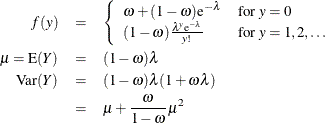
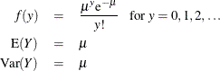
Poisson Distribution
Tweedie Distribution
The Tweedie model is a generalized linear model from the exponential family. The Tweedie distribution is characterized by
three parameters: the mean parameter  , the dispersion
  , and the power p. The variance of the distribution is
  . For values of p in the range
  , a Tweedie random variable can be represented as a Poisson sum of gamma distributed random variables. That is,
![\[ Y = \sum _{i=1}^{N}Y_ i \]](images/stathpug_hpgenselect0080.png)
where N has a Poisson distribution
that has mean  and the
  have independent, identical gamma distributions
, each of which has an expected value
have independent, identical gamma distributions
, each of which has an expected value 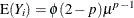 and an index parameter
  .
.
In this case, Y has a discrete mass at 0,  , and the probability density of Y
  is represented by an infinite series for
  . The HPGENSELECT procedure restricts the power parameter to satisfy
  for numerical stability in model fitting. The Tweedie distribution does not have a general closed form representation for
all values of p. It can be characterized in terms of the distribution mean parameter , dispersion parameter , and power parameter p. For more information about the Tweedie distribution, see Frees (2010).
for numerical stability in model fitting. The Tweedie distribution does not have a general closed form representation for
all values of p. It can be characterized in terms of the distribution mean parameter , dispersion parameter , and power parameter p. For more information about the Tweedie distribution, see Frees (2010).
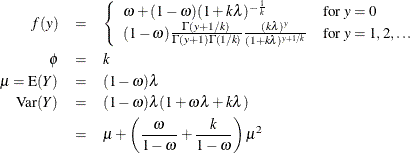
The distribution mean and variance are given by:
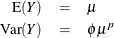
Zero-Inflated Negative Binomial Distribution
For the zero-inflated negative binomial distribution, k is the estimated dispersion parameter that is displayed in the output.
Zero-Inflated Poisson Distribution