The HPQUANTSELECT Procedure

Example 13.1 Simulation Study

This example is based on Simulation Study in SAS/STAT 13.2 User's Guide. This simulation study shows how you can use the forward selection method to select quantile regression models for single quantile levels. The following statements simulate a data set from a naive instrumental model (Chernozhukov and Hansen, 2008):

%let seed=321;
%let p=20;
%let n=3000;

data analysisData;
   array x{&p} x1-x&p;
   do i=1 to &n;
      U  = ranuni(&seed);
      x1 = ranuni(&seed);
      x2 = ranexp(&seed);
      x3 = abs(rannor(&seed));
      y  = x1*(U-0.1) + x2*(U*U-0.25) + x3*(exp(U)-exp(0.9));
      do j=4 to &p;
         x{j} = ranuni(&seed);
      end;
      output;
   end;
run;

Variable U in the data set indicates the true quantile level of the response y conditional on $\mb{x}=(x_1,\ldots ,x_ p)$ .

Let $Q_ Y(\tau |\mb{x})=\mb{x} {\mbox{\boldmath $\beta $}}(\tau )$ denote the underlying quantile regression model, where ${\mbox{\boldmath $\beta $}}(\tau )=(\beta _1(\tau ),\ldots ,\beta _ p(\tau ))’$ . Then, the true parameter functions are

$\begin{eqnarray*} \beta _1(\tau )& =& \tau -0.1\\ \beta _2(\tau )& =& \tau ^2-0.25\\ \beta _3(\tau )& =& \exp (\tau )-\exp (0.9)\\ \beta _4(\tau )& =& \cdots =\beta _ p(\tau )=0 \end{eqnarray*}$

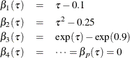
It is easy to see that, at $\tau =0.1$ , only $\beta _2(0.1)=-0.24$ and $\beta _3(0.1)=\exp (0.1)-\exp (0.9)\approx -1.354432$ are nonzero parameters. Therefore, an effective effect-selection method should select x2 and x3 and drop all the other effects in this data set at $\tau =0.1$ . By the same rationale, x1 and x3 should be selected at $\tau =0.5$ with $\beta _1(0.5)=0.4$ and $\beta _3(0.5)\approx -0.810882$ , and x1 and x2 should be selected at $\tau =0.9$ with $\beta _1(0.9)=0.8$ and $\beta _2(0.9)=0.56$ .

The following statements use PROC HPQUANTSELECT with the forward selection method. The STB option and the CLB option in the MODEL statement request the standardized parameter estimates and the confidence limits of parameter estimates, respectively.

proc hpquantselect data=analysisData;
   model y= x1-x&p / quantile=0.1 0.5 0.9 stb clb;
   selection method=forward;
   output out=out p=pred;
run;

Output 13.1.1 shows that, by default, the CHOOSE= and STOP= options are both set to SBC.

Output 13.1.1: Model Information

The HPQUANTSELECT Procedure

Selection Information
Selection Method	Forward
Select Criterion	SBC
Stop Criterion	SBC
Effect Hierarchy Enforced	None
Stop Horizon	3

Output 13.1.2, Output 13.1.3, and Output 13.1.4 display the selected effects and the parameter estimates for $\tau =0.1$ , $\tau =0.5$ , and $\tau =0.9$ , respectively. You can see that the forward selection method correctly selects active effects for all three quantile levels.

Output 13.1.2: Parameter Estimates at $\tau =0.1$

The HPQUANTSELECT Procedure

Quantile Level = 0.1

Selected Model

Selected Effects:	Intercept x2 x3

Parameter Estimates
Parameter	DF	Estimate	Standardized Estimate	Standard Error	95% Confidence Limits
Intercept	1	0.01179	0	0.01192	-0.01158	0.03516
x2	1	-0.22871	-0.21829	0.00946	-0.24725	-0.21017
x3	1	-1.37991	-0.78452	0.01556	-1.41042	-1.34939

Output 13.1.3: Parameter Estimates at $\tau =0.5$

The HPQUANTSELECT Procedure

Quantile Level = 0.5

Selected Model

Selected Effects:	Intercept x1 x3

Parameter Estimates
Parameter	DF	Estimate	Standardized Estimate	Standard Error	95% Confidence Limits
Intercept	1	0.01178	0	0.03418	-0.05524	0.07879
x1	1	0.42584	0.11879	0.06237	0.30355	0.54814
x3	1	-0.86332	-0.49082	0.04765	-0.95674	-0.76989

Output 13.1.4: Parameter Estimates at $\tau =0.9$

The HPQUANTSELECT Procedure

Quantile Level = 0.9

Selected Model

Selected Effects:	Intercept x1 x2

Parameter Estimates
Parameter	DF	Estimate	Standardized Estimate	Standard Error	95% Confidence Limits
Intercept	1	-0.00774	0	0.03292	-0.07228	0.05680
x1	1	0.78294	0.21841	0.05134	0.68228	0.88360
x2	1	0.57644	0.55018	0.03422	0.50935	0.64354