The HPLOGISTIC Procedure
-
Overview

-
Getting Started
-
Syntax
-
DetailsMissing ValuesResponse DistributionsLog-Likelihood FunctionsExistence of Maximum Likelihood EstimatesUsing Validation and Test DataModel Fit and Assessment StatisticsThe Hosmer-Lemeshow Goodness-of-Fit TestComputational Method: MultithreadingChoosing an Optimization AlgorithmDisplayed OutputODS Table Names
-
Examples
- References
If ![]() are independent binary (Bernoulli) random variables with common success probability
are independent binary (Bernoulli) random variables with common success probability ![]() , then their sum is a binomial random variable. In other words, a binomial random variable with parameters n and
, then their sum is a binomial random variable. In other words, a binomial random variable with parameters n and ![]() can be generated as the sum of n Bernoulli(
can be generated as the sum of n Bernoulli(![]() ) random experiments. The HPLOGISTIC procedure uses a special syntax to express data in binomial form, the events/trials syntax.
) random experiments. The HPLOGISTIC procedure uses a special syntax to express data in binomial form, the events/trials syntax.
Consider the following data, taken from Cox and Snell (1989, pp. 10–11), of the number, r, of ingots not ready for rolling, out of n tested, for a number of combinations of heating time and soaking time. If each test is carried out independently and if for
a particular combination of heating and soaking time there is a constant probability that the tested ingot is not ready for
rolling, then the random variable r follows a Binomial![]() distribution, where the success probability
distribution, where the success probability ![]() is a function of heating and soaking time.
is a function of heating and soaking time.
data Ingots;
   input Heat Soak r n @@;
   Obsnum= _n_;
   datalines;
7 1.0 0 10  14 1.0 0 31  27 1.0 1 56  51 1.0 3 13
7 1.7 0 17  14 1.7 0 43  27 1.7 4 44  51 1.7 0  1
7 2.2 0  7  14 2.2 2 33  27 2.2 0 21  51 2.2 0  1
7 2.8 0 12  14 2.8 0 31  27 2.8 1 22  51 4.0 0  1
7 4.0 0  9  14 4.0 0 19  27 4.0 1 16
;
The following statements show the use of the events/trials syntax to model the binomial response. The events variable in this situation is r, the number of ingots not ready for rolling, and the trials variable is n, the number of ingots tested. The dependency of the probability of not being ready for rolling is modeled as a function of
heating time, soaking time, and their interaction. The ASSOCIATION
option displays ordinal measures of association between the observed responses and predicted probabilities. The CTABLE=
ROC option stores statistics that are used for evaluating the predictive power of the model in the Roc data set. The LACKFIT
option produces the Hosmer and Lemeshow goodness-of-fit test for binary response models. The OUTPUT
statement stores the linear predictors and the predicted probabilities in the Out data set along with the ID
variable.
proc hplogistic data=Ingots;
   model r/n = Heat Soak Heat*Soak / association ctable=Roc lackfit;
   id Obsnum;
   output out=Out xbeta predicted=Pred;
run;
The "Performance Information" table in Output 9.2.1 shows that the procedure executes in single-machine mode. The example is executed on a single machine with the same number of cores as the number of threads used; that is, one computational thread was spawned per CPU.
The "Model Information" table shows that the data are modeled as binomially distributed with a logit link function (Output 9.2.2). This is the default link function in the HPLOGISTIC procedure for binary and binomial data. The procedure estimates the parameters of the model by a Newton-Raphson algorithm.
The second table in Output 9.2.2 shows that all 19 observations in the data set were used in the analysis, and that the total number of events and trials
equal 12 and 387, respectively. These are the sums of the variables r and n across all observations.
Output 9.2.3 displays the "Iteration History" and convergence status tables for this run. The HPLOGISTIC procedure converged after four iterations (not counting the initial setup iteration) and meets the GCONV= convergence criterion.
Output 9.2.4 displays the "Dimensions" table for the model. There are four columns in the design matrix of the model (the ![]() matrix); they correspond to the intercept, the
matrix); they correspond to the intercept, the Heat effect, the Soak effect, and the interaction of the Heat and Soak effects. The model is nonsingular, since the rank of the crossproducts matrix equals the number of columns in ![]() . All parameters are estimable and participate in the optimization.
. All parameters are estimable and participate in the optimization.
Output 9.2.5 displays the "Fit Statistics" table for this run. Evaluated at the converged estimates, –2 times the value of the log-likelihood function equals 27.9569. Further fit statistics are also given, all of them in "smaller is better" form. The AIC, AICC, and BIC criteria are used to compare non-nested models and to penalize the model fit for the number of observations and parameters. The –2 log-likelihood value can be used to compare nested models by way of a likelihood ratio test.
Output 9.2.6 shows the test of the global hypothesis that the effects jointly do not impact the probability of ingot readiness. The chi-square test statistic can be obtained by comparing the –2 log-likelihood value of the model with covariates to the value in the intercept-only model. The test is significant with a p-value of 0.0082. One or more of the effects in the model have a significant impact on the probability of ingot readiness.
Output 9.2.7 shows the tables that are produced when you specify the LACKFIT option in the MODEL statement. The first table displays the partition that PROC HPLOGISTIC uses to compute the chi-square test that is displayed in the second table; the large p-value does not reject the adequacy of the model fit. For more information, see the section The Hosmer-Lemeshow Goodness-of-Fit Test.
Output 9.2.7: Hosmer-Lemeshow Goodness-of-Fit Test
| Partition for the Hosmer and Lemeshow Test | |||||
|---|---|---|---|---|---|
| Group | Events | Nonevents | Total | ||
| Observed | Expected | Observed | Expected | ||
| 1 | 0 | 0.24 | 34 | 33.76 | 34 |
| 2 | 0 | 0.47 | 43 | 42.53 | 43 |
| 3 | 0 | 0.66 | 52 | 51.34 | 52 |
| 4 | 2 | 0.46 | 31 | 32.54 | 33 |
| 5 | 0 | 0.48 | 31 | 30.52 | 31 |
| 6 | 0 | 0.36 | 19 | 18.64 | 19 |
| 7 | 1 | 1.94 | 55 | 54.06 | 56 |
| 8 | 4 | 1.59 | 40 | 42.41 | 44 |
| 9 | 1 | 1.63 | 42 | 41.37 | 43 |
| 10 | 4 | 4.17 | 28 | 27.83 | 32 |
Output 9.2.8 displays the "Association Statistics" table, which is produced when you specify the ASSOCIATION option in the MODEL statement. The table contains four measures of association for assessing the predictive ability of a model. For more information, see the section Association Statistics.
The "Parameter Estimates" table in Output 9.2.9 displays the estimates and standard errors of the model effects.
You can construct the prediction equation of the model from the "Parameter Estimates" table. For example, an observation with
Heat equal to 14 and Soak equal to 1.7 has linear predictor
The probability that an ingot with these characteristics is not ready for rolling is
The OUTPUT
statement computes these linear predictors and probabilities and stores them in the Out data set. This data set also contains the ID variable, which is used by the following statements to attach the covariates
to these statistics. Output 9.2.10 shows the probability that an ingot with Heat equal to 14 and Soak equal to 1.7 is not ready for rolling.
data Out;
   merge Out Ingots;
   by Obsnum;
proc print data=Out;
   where Heat=14 & Soak=1.7;
run;
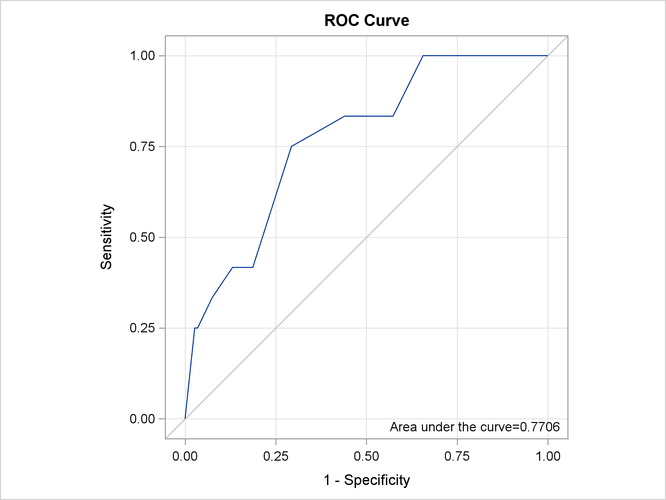
The CTABLE=
ROC option computes statistics for binary response models (based on classifying observations according to whether their predicted
probabilities exceed certain values) and stores the results in the Roc data set. For more information, see the section Classification Table and ROC Curves. You can use this data set to display the ROC curve by using the SGPLOT procedure as follows:
proc sgplot data=Roc aspect=1 noautolegend;
   title 'ROC Curve';
   xaxis values=(0 to 1 by 0.25) grid offsetmin=.05 offsetmax=.05;
   yaxis values=(0 to 1 by 0.25) grid offsetmin=.05 offsetmax=.05;
   lineparm x=0 y=0 slope=1 / lineattrs=(color=ligr);
   series x=FPF y=TPF;
   inset 'Area under the curve=0.7706' / position=bottomright;
run;
Binomial data are a form of grouped binary data where "successes" in the underlying Bernoulli trials are totaled. You can thus unwind data for which you use the events/trials syntax and fit it with techniques for binary data.
The following DATA step expands the Ingots data set with 12 events in 387 trials into a binary data set with 387 observations.
data Ingots_binary;
   set Ingots;
   do i=1 to n;
     if i <= r then y=1; else y = 0;
     output;
   end;
run;
The following HPLOGISTIC statements fit the model with Heat effect, Soak effect, and their interaction to the binary data set. The event=’1’ response-variable option in the MODEL
statement ensures that the HPLOGISTIC procedure models the probability that the variable y takes on the value ('1').
proc hplogistic data=Ingots_binary;
   model y(event='1') = Heat Soak Heat*Soak;
run;
Output 9.2.12 displays the "Performance Information", "Model Information," "Number of Observations," and the "Response Profile" tables.
The data are now modeled as binary (Bernoulli distributed) with a logit link function. The "Response Profile" table shows
that the binary response breaks down into 375 observations where y equals zero and 12 observations where y equals 1.
Output 9.2.13 displays the result for the test of the global null hypothesis and the parameter estimates. These results match those in Output 9.2.6 and Output 9.2.9.