The HPGENSELECT Procedure

The HPGENSELECT procedure forms the log-likelihood functions of the various models as
where ![]() is the log-likelihood contribution of the ith observation that has weight
is the log-likelihood contribution of the ith observation that has weight ![]() , and
, and ![]() is the value of the frequency variable. For the determination of
is the value of the frequency variable. For the determination of ![]() and
and ![]() , see the WEIGHT
and FREQ
statements. The individual log-likelihood contributions for the various distributions are as follows.
, see the WEIGHT
and FREQ
statements. The individual log-likelihood contributions for the various distributions are as follows.
In the following, the mean parameter ![]() for each observation i is related to the regression parameters
for each observation i is related to the regression parameters ![]() through the linear predictor
through the linear predictor ![]() by
by
where g is the link function.
There are two link functions and linear predictors that are associated with zero-inflated Poisson and zero-inflated negative
binomial distributions: one for the zero-inflation probability ![]() , and another for the parameter
, and another for the parameter ![]() , which is the Poisson or negative binomial mean if there is no zero-inflation. Each of these parameters is related to regression
parameters through an individual link function,
, which is the Poisson or negative binomial mean if there is no zero-inflation. Each of these parameters is related to regression
parameters through an individual link function,
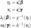
where h is one of the following link functions that are associated with binary data: complementary log-log, log-log, logit, or probit. These link functions are also shown in Table 7.9.
The HPGENSELECT procedure computes the log-likelihood function ![]() for the ith binary observation as
for the ith binary observation as
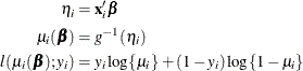
Here, ![]() is the probability of an event, and the variable
is the probability of an event, and the variable ![]() takes on the value 1 for an event and the value 0 for a non-event. The inverse link function
takes on the value 1 for an event and the value 0 for a non-event. The inverse link function ![]() maps from the scale of the linear predictor
maps from the scale of the linear predictor ![]() to the scale of the mean. For example, for the logit link (the default),
to the scale of the mean. For example, for the logit link (the default),
You can control which binary outcome in your data is modeled as the event by specifying the response-options in the MODEL statement, and you can choose the link function by specifying the LINK= option in the MODEL statement.
If a WEIGHT
statement is specified and ![]() denotes the weight for the current observation, the log-likelihood function is computed as
denotes the weight for the current observation, the log-likelihood function is computed as
The HPGENSELECT procedure computes the log-likelihood function ![]() for the ith binomial observation as
for the ith binomial observation as
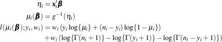
where ![]() and
and ![]() are the values of the events and trials of the ith observation, respectively.
are the values of the events and trials of the ith observation, respectively. ![]() measures the probability of events (successes) in the underlying Bernoulli distribution whose aggregate follows the binomial
distribution.
measures the probability of events (successes) in the underlying Bernoulli distribution whose aggregate follows the binomial
distribution.
The HPGENSELECT procedure computes the log-likelihood function ![]() for the ith observation as
for the ith observation as
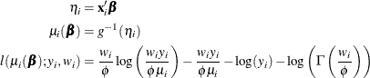
For the gamma distribution, ![]() is the estimated dispersion parameter that is displayed in the output.
is the estimated dispersion parameter that is displayed in the output.
The HPGENSELECT procedure computes the log-likelihood function ![]() for the ith observation as
for the ith observation as
![\begin{align*} \eta _ i & = \mb{x}_ i’\bbeta \\ \mu _ i(\bbeta ) & = g^{-1}(\eta _ i) \\ l(\mu _ i(\bbeta );y_ i,w_ i) & = -\frac{1}{2} \left[ \frac{w_ i(y_ i-\mu _ i)^2}{y_ i \mu ^2 \phi } + \log \left( \frac{\phi y_ i^3}{w_ i} \right) + \log (2 \pi ) \right] \end{align*}](images/stathpug_hpgenselect0103.png)
where ![]() is the dispersion parameter.
is the dispersion parameter.
The multinomial distribution that is modeled by the HPGENSELECT procedure is a generalization of the binary distribution; it is the distribution of a single draw from a discrete distribution with J possible values. The log-likelihood function for the ith observation is
In this expression, J denotes the number of response categories (the number of possible outcomes) and ![]() is the probability that the ith observation takes on the response value that is associated with category j. The category probabilities must satisfy
is the probability that the ith observation takes on the response value that is associated with category j. The category probabilities must satisfy
and the constraint is satisfied by modeling ![]() categories. In models that have ordered response categories, the probabilities are expressed in cumulative form, so that
the last category is redundant. In generalized logit models (multinomial models that have unordered categories), one category
is chosen as the reference category and the linear predictor in the reference category is set to 0.
categories. In models that have ordered response categories, the probabilities are expressed in cumulative form, so that
the last category is redundant. In generalized logit models (multinomial models that have unordered categories), one category
is chosen as the reference category and the linear predictor in the reference category is set to 0.
The HPGENSELECT procedure computes the log-likelihood function ![]() for the ith observation as
for the ith observation as
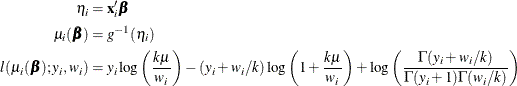
where k is the negative binomial dispersion parameter that is displayed in the output.
The HPGENSELECT procedure computes the log-likelihood function ![]() for the ith observation as
for the ith observation as
![\begin{align*} \eta _ i & = \mb{x}_ i’\bbeta \\ \mu _ i(\bbeta ) & = g^{-1}(\eta _ i) \\ l(\mu _ i(\bbeta );y_ i,w_ i) & = -\frac{1}{2} \left[ \frac{w_ i(y_ i-\mu _ i)^2}{\phi } + \log \left( \frac{\phi }{w_ i} \right) + \log (2 \pi ) \right] \end{align*}](images/stathpug_hpgenselect0108.png)
where ![]() is the dispersion parameter.
is the dispersion parameter.
The HPGENSELECT procedure computes the log-likelihood function ![]() for the ith observation as
for the ith observation as
![\begin{align*} \eta _ i & = \mb{x}_ i’\bbeta \\ \mu _ i(\bbeta ) & = g^{-1}(\eta _ i) \\ l(\mu _ i(\bbeta );y_ i,w_ i) & = w_ i[y_ i \log (\mu _ i) - \mu _ i - \log (y_ i!) ] \end{align*}](images/stathpug_hpgenselect0109.png)
The Tweedie distribution does not in general have a closed form log-likelihood function in terms of the mean, dispersion, and power parameters. The form of the log likelihood is
where
and ![]() is the Tweedie probability distribution, which is described in the section Tweedie Distribution. Evaluation of the Tweedie log-likelihood for model fitting is performed numerically as described in Dunn and Smyth (2005, 2008).
is the Tweedie probability distribution, which is described in the section Tweedie Distribution. Evaluation of the Tweedie log-likelihood for model fitting is performed numerically as described in Dunn and Smyth (2005, 2008).
The extended quasi-likelihood (EQL) is constructed according to the definition of McCullagh and Nelder (1989, Chapter 9) as
where the contribution from an observation is
where ![]() . This EQL is used in computing initial values for the iterative maximization of the Tweedie log likelihood, as specified
using the OPTMETHOD= Tweedie option in Table 7.5. If you specify the OPTMETHOD=EQL Tweedie-optimization-option in Table 7.5, then the parameter estimates are computed by using the EQL instead of the log likelihood.
. This EQL is used in computing initial values for the iterative maximization of the Tweedie log likelihood, as specified
using the OPTMETHOD= Tweedie option in Table 7.5. If you specify the OPTMETHOD=EQL Tweedie-optimization-option in Table 7.5, then the parameter estimates are computed by using the EQL instead of the log likelihood.
The HPGENSELECT procedure computes the log-likelihood function ![]() for the ith observation as
for the ith observation as
![\begin{align*} \eta _ i & = \mb{x}_ i’\bbeta \\ \kappa _ i & = \mb{z}_ i^\prime \bgamma \\ \lambda _ i(\bbeta ) & = g^{-1}(\eta _ i) \\ \omega _ i(\bgamma ) & = h^{-1}(\kappa _ i)\\ l(\mu _ i(\bbeta ),\omega _ i(\bgamma );y_ i,w_ i) & = \left\{ \begin{array}{ll} \log [\omega _ i + (1-\omega _ i)(1+\frac{k}{w_ i}\lambda )^{-\frac{1}{k}}] & y_ i=0 \\ \log (1-\omega _ i)+ y_ i\log \left(\frac{k\lambda }{w_ i} \right) & \\ -(y_ i+\frac{w_ i}{k})\log \left(1+\frac{k\lambda }{w_ i} \right) & \\ +\log \left(\frac{\Gamma (y_ i+\frac{w_ i}{k})}{\Gamma (y_ i+1)\Gamma (\frac{w_ i}{k})}\right) & y_ i>0 \\ \end{array} \right. \end{align*}](images/stathpug_hpgenselect0115.png)
where k is the zero-inflated negative binomial dispersion parameter that is displayed in the output.
![\begin{align*} \eta _ i & = \mb{x}_ i’\bbeta \\ \kappa _ i & = \mb{z}_ i^\prime \bgamma \\ \lambda _ i(\bbeta ) & = g^{-1}(\eta _ i) \\ \omega _ i(\bgamma ) & = h^{-1}(\kappa _ i)\\ l(\mu _ i(\bbeta ),\omega _ i(\bgamma );y_ i,w_ i) & = \left\{ \begin{array}{ll} w_ i\log [\omega _ i + (1-\omega _ i)\exp (-\lambda _ i)] & y_ i=0 \\ w_ i[\log (1-\omega _ i)+y_ i \log (\lambda _ i) - \lambda _ i-\log (y_ i!)] & y_ i>0 \\ \end{array} \right. \end{align*}](images/stathpug_hpgenselect0116.png)