Example 7.1 Segmented Model :: SAS/STAT(R) 12.3 User's Guide: High-Performance Procedures

Example 7.1 Segmented Model

Suppose you are interested in fitting a model that consists of two segments that connect in a smooth fashion. For example, the following model states that the mean of is a quadratic function in for values of less than and that the mean of is constant for values of greater than :

$\mr {E}[Y|x] = \left\{ \begin{array}{ll} \alpha + \beta x + \gamma x^2 & \quad \mr {if} \, \, \, x < x_0 \cr c & \quad \mr {if} \, \, \, x \ge x_0 \end{array} \right.$

In this model equation, $\alpha$ , $\beta$ , and $\gamma$ are the coefficients of the quadratic segment, and is the plateau of the mean function. The HPNLMOD procedure can fit such a segmented model even when the join point, , is unknown.

Suppose you also want to impose conditions on the two segments of the model. First, the curve should be continuous—that is, the quadratic and the plateau section need to meet at . Second, the curve should be smooth—that is, the first derivative of the two segments with respect to needs to coincide at .

The continuity condition requires that

$c = \mr {E}[Y|x_0] = \alpha + \beta x_0 + \gamma x_0^2$

The smoothness condition requires that

$\frac{\partial \mr {E}[Y|x_0]}{\partial x} = \beta + 2\gamma x_0 \equiv 0$

If you solve for and substitute into the expression for , the two conditions jointly imply that

$\displaystyle x_0$	$\displaystyle = - \beta / 2 \gamma$
$\displaystyle c$	$\displaystyle = \alpha - \beta ^2 / 4 \gamma$

Although there are five unknowns, the model contains only three independent parameters. The continuity and smoothness restrictions together completely determine two parameters, given the other three.

The following DATA step creates the SAS data set for this example:

data a;
   input y x @@;
   datalines;
.46 1  .47  2 .57  3 .61  4 .62  5 .68  6 .69  7
.78 8  .70  9 .74 10 .77 11 .78 12 .74 13 .80 13
.80 15 .78 16
 ;

The following PROC HPNLMOD statements fit this segmented model:

proc hpnlmod data=a out=b;
   parms alpha=.45 beta=.05 gamma=-.0025;
   
   x0 = -.5*beta / gamma;
   
   if (x < x0) then 
        yp = alpha + beta*x  + gamma*x*x;
   else 
        yp = alpha + beta*x0 + gamma*x0*x0;

   model y ~ residual(yp);

   estimate 'join point' -beta/2/gamma;
   estimate 'plateau value c' alpha - beta**2/(4*gamma);
   predict 'predicted' yp pred=yp;
   predict 'response' y pred=y;
   predict 'x' x pred=x;
run;

The parameters of the model are $\alpha$ , $\beta$ , and $\gamma$ . They are represented in the PROC HPNLMOD statements by the variables alpha, beta, and gamma, respectively. In order to model the two segments, a conditional statement assigns the appropriate expression to the mean function, depending on the value of . The ESTIMATE statements compute the values of and . The PREDICT statement computes predicted values for plotting and saves them to data set b.

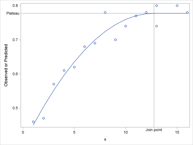
The results from fitting this model are shown in Output 7.1.1 through Output 7.1.3. The iterative optimization converges after six iterations (Output 7.1.1). Output 7.1.2 shows the estimated parameters. Output 7.1.3 indicates that the join point is and the plateau value is .

Output 7.1.1: Nonlinear Least Squares Iterative Phase

Quadratic Model with Plateau

The HPNLMOD Procedure

Iteration History
Iteration	Evaluations	Objective Function	Change	Max Gradient
0	5	0.0035144531		7.184063
1	2	0.0007352716	0.00277918	2.145337
2	2	0.0006292751	0.00010600	0.032551
3	2	0.0006291261	0.00000015	0.002952
4	2	0.0006291244	0.00000000	0.000238
5	2	0.0006291244	0.00000000	0.000023
6	2	0.0006291244	0.00000000	2.313E-6

Convergence criterion (GCONV=1E-8) satisfied.

Output 7.1.2: Least Squares Analysis for the Quadratic Model

Analysis of Variance
Source	DF	Sum of Squares	Mean Square	F Value	Approx Pr > F
Model	2	0.1769	0.0884	114.22	<.0001
Error	13	0.0101	0.000774
Corrected Total	15	0.1869

Parameter Estimates
Parameter	Estimate	Standard Error	DF	t Value	Approx Pr > \|t\|	Approximate 95% Confidence Limits
alpha	0.3921	0.0267	1	14.70	<.0001	0.3345	0.4497
beta	0.0605	0.00842	1	7.18	<.0001	0.0423	0.0787
gamma	-0.00237	0.000551	1	-4.30	0.0009	-0.00356	-0.00118

Output 7.1.3: Additional Estimates for the Quadratic Model

Additional Estimates
Label	Estimate	Standard Error	DF	t Value	Approx Pr > \|t\|	Alpha	Approximate Confidence Limits
join point	12.7477	1.2781	1	9.97	<.0001	0.05	9.9864	15.5089
plateau value c	0.7775	0.0123	1	63.11	<.0001	0.05	0.7509	0.8041

The following statements produce a graph of the observed and predicted values along with reference lines for the join point and plateau estimates (Output 7.1.4):

proc sgplot data=b noautolegend;
   yaxis label='Observed or Predicted';
   refline 0.7775  / axis=y label="Plateau"    labelpos=min;
   refline 12.7477 / axis=x label="Join point" labelpos=min;
   scatter y=y  x=x;
   series  y=yp x=x;
run;

Output 7.1.4: Observed and Predicted Values for the Quadratic Model