Residual-by-Hat Diagonal Plot

Multiple Regression

Residual-by-Hat Diagonal Plot

The fit window contains additional diagnostic tools for examining the effect of observations. One such tool is the residual-by-hat diagonal plot. Hat diagonal refers to the diagonal elements of the hat matrix (Rawlings 1988). Hat diagonal measures the leverage of each observation on the predicted value for that observation.

Choosing Fit (Y X) does not automatically generate the residual-by-hat diagonal plot, but you can easily add it to the fit window. First, add the hat diagonal variable to the data window.

Choose Vars:Hat Diag.

[menu]
Figure 14.10: Vars Menu

This adds the variable H_GPA to the data window, as shown in Figure 14.11. (The residual variable, R_GPA, is added when a residual-by-predicted plot is created.)

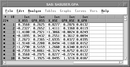
Figure 14.11: GPA Data Window with H_GPA Added

Drag a rectangle in the fit window to select an area for the new plot.

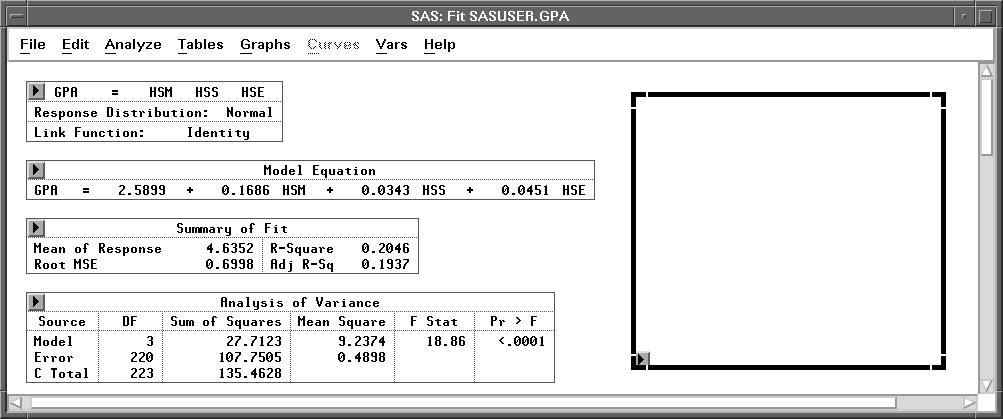
Figure 14.12: Selecting an Area

Choose Analyze:Scatter Plot (Y X).

[menu]
Figure 14.13: Analyze Menu

This displays the scatter plot variables dialog.

Assign R_GPA the Y role and H_GPA the X role, then click on OK.

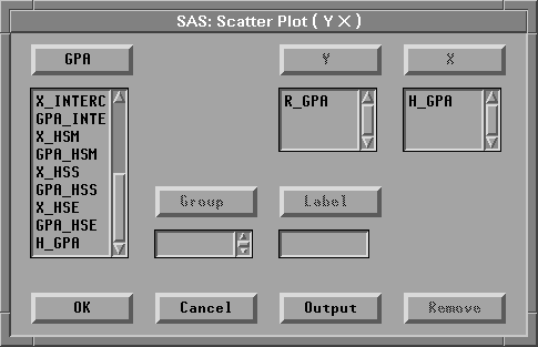
Figure 14.14: Scatter Plot Variables Dialog

The plot appears in the fit window in the area you selected.

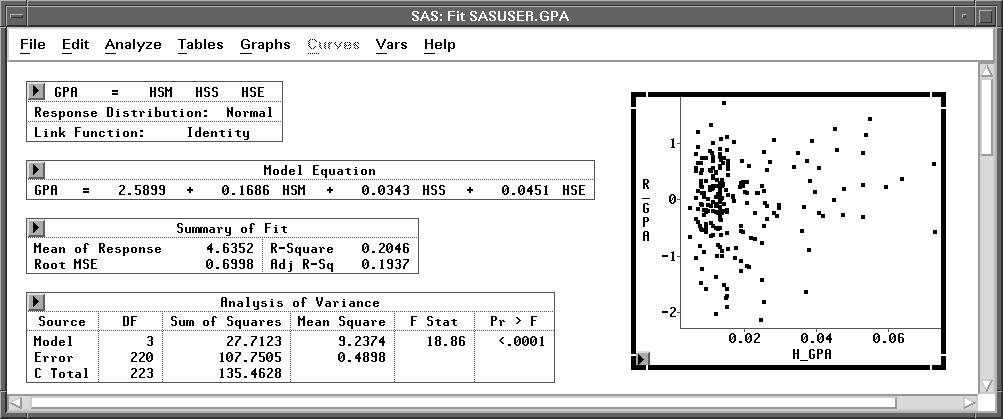
Figure 14.15: Residual by Hat Diagonal Plot

Belsley, Kuh, and Welsch (1980) propose a cutoff of 2 p/ n for the hat diagonal values, where n is the number of observations used to fit the model and p is the number of parameters in the model. Observations with values above this cutoff should be investigated. For this example, H_GPA values over 0.036 should be investigated. About 15% of the observations have values above this cutoff.

There are other measures you can use to determine the influence of observations. These include Cook's D, Dffits, Covratio, and Dfbetas. Each of these measures examines some effect of deleting the ith observation.

Choose Vars:Dffits.

A new variable, F_GPA, that contains the Dffits values is added to the data window.

Large absolute values of Dffits indicate influential observations. A general cutoff to consider is 2. It is, thus, useful in this example to identify those observations where H_GPA exceeds 0.036 and the absolute value of F_GPA is greater than 2. One way to accomplish this is by examining the H_GPA by F_GPA scatter plot.

Choose Analyze:Scatter Plot (Y X).

This displays the scatter plot variables dialog.

Assign H_GPA the Y role and F_GPA the X role, then click on OK.

This displays the H_GPA by F_GPA scatter plot.

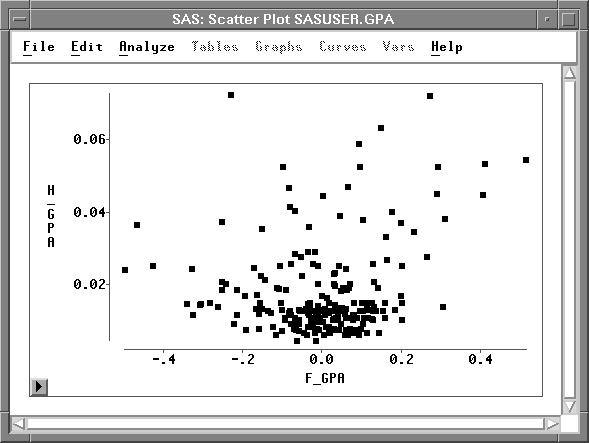
Figure 14.16: H_GPA by F_GPA Scatter Plot

None of the observations identified as potential influential observations (H_GPA > 0.036) are, in fact, influential for this model using the criterion ${{|{\hvb F\_GPA}|} \gt 2}$ .

Top of Page