Poisson Regression

Displaying the Poisson Regression Analysis

The SHIP data shown in Figure 17.2 represent damage caused by waves to the forward section of certain cargo-carrying vessels. The purpose of the investigation was to set standards for future hull construction. In order to do so, the investigators needed to know the risk of damage associated with five ship types (TYPE), year of construction (YEAR), and period of operation (PERIOD). These three variables are the classification variables. MONTHS is the aggregate number of months in service and is an explanatory variable. Y is the response variable and represents the number of damage incidents (McCullagh and Nelder 1989).

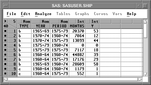
Figure 17.2: SHIP Data Set

Recall from Chapter 16 that the generalized linear model has three basic components:

a linear function of explanatory variables. For this example, the function is

${ {\beta}_{0} + {\beta}_{1} \log({MONTHS}) + {\gamma}_{i} + {\tau}_{j} + {\de... ...k} + ({\gamma}{\tau})_{ij} + ({\gamma}{\delta})_{ik} + ({\tau}{\delta})_{jk}}$

where log( MONTHS) is a variable whose coefficient ${\beta}$ ₁ is believed to be 1. An effect such as this is commonly referred to as an offset. ${{\gamma}_{i}}$ is the effect of the ith level of TYPE, ${{\tau}_{j}}$ is the effect of the jth level of YEAR, ${{\delta}_{k}}$ is the effect of the kth level of PERIOD, ${({\gamma}{\tau})_{ij}}$ is the effect of the ijth level of the TYPE by YEAR interaction, ${({\gamma}{\delta})_{ik}}$ is the effect of the ikth level of the TYPE by PERIOD interaction, and ${({\tau}{\delta})_{jk}}$ is the effect of the jkth level of the YEAR by PERIOD interaction.
a probability function for the response variable that depends on the mean and sometimes other parameters as well. For this example, the probability function of the response variable is Poisson.
a link function that relates the mean to the linear function of explanatory variables. For this example, the link function is the log

<<I>br>log( expected number of damage incidents)

$= \hspace*{.2in}{ {\beta}_{0} + {\beta}_{1} \log({MONTHS}) + {\gamma}_{i} + {\... ...k} + ({\gamma}{\tau})_{ij} + ({\gamma}{\delta})_{ik} + ({\tau}{\delta})_{jk}}$

Open the SHIP data set.

Recall from the previous equation that Y is assumed to be directly proportional to MONTHS. Since log(Y) is being modeled, you need to carry out a log transformation on MONTHS. Follow these steps to create a new variable that represents the log of MONTHS.

Select MONTHS in the data window.

Choose Edit:Variables:log( Y ).

[menu]

Figure 17.3: Edit:Variables Menu

A new variable, L_MONTHS, now appears in the data window.

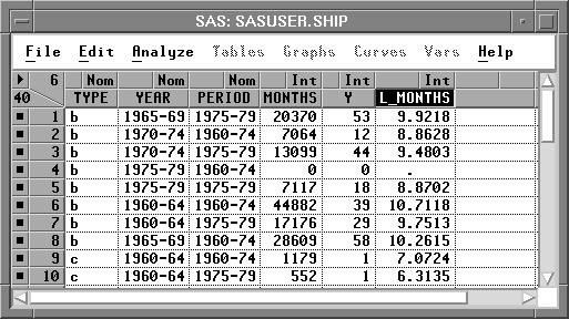
Figure 17.4: Data Window with L_MONTHS Added

Deselect L_MONTHS in the data window.

Some values of MONTHS are 0, meaning that this kind of ship has not seen service. You need to restrict these observations from entering into the model fit. The log transformation does this automatically since log(MONTHS) becomes a missing value for the observations with a value of 0 for MONTH. Observations with missing values for the explanatory variables or the response variable are not used in the model fit.

Now you are ready to begin the analysis.

Choose Analyze:Fit ( Y X ) to display the fit variables dialog

Select Y in the list at the left, then click the Y button.

Y appears in the Y variables list.

Select TYPE, YEAR, and PERIOD, then click the Expand button.

TYPE, YEAR, and PERIOD, along with all two-way interaction effects, appear in the X variables list. Your variables dialog should now appear as shown in Figure 17.5.

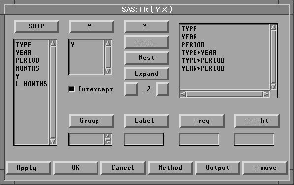
Figure 17.5: Fit Variables Dialog with Variable Roles Assigned

The Expand button provides a convenient way to specify interactions of any order. The order 2 is the default. You can change the order by entering a different value to replace the 2 or by clicking on the buttons to the right or left of the 2 to increase or decrease the order, respectively.

Click the Method button to display the fit method dialog

This dialog enables you to specify the probability function or the quasi-likelihood function for the response variable and the link function.

Overdispersion is a phenomenon that occurs occasionally with binomial and Poisson data. For Poisson data, it occurs when the variance of the response Y exceeds the Poisson variance Var(y)= ${\mu}$ .To account for the overdispersion that might occur in the SHIP data set, a quasi-likelihood function with variance function Var( ${\mu}$ )= ${\mu}$ (Poisson variance) will be used for the response variable. The variance is given by

$\rm{Var}(y) = {\sigma}^2 {\mu}$

where ${\sigma}$ ² is the dispersion parameter with value greater than 1 for overdispersion.

Select the check box for Quasi-Likelihood.

Click on Poisson under Response Dist.

This uses the Poisson variance function Var( ${\mu}$ ) = ${\mu}$ for the quasi-likelihood function.

Click on Pearson under Scale.

This uses the scale parameter based on the Pearson ${\chi}$ ² statistic.

Select L_MONTHS in the list at the left, then click the Offset button.

L_MONTHS appears in the Offset variables list. Your method dialog should now appear as shown in Figure 17.6.

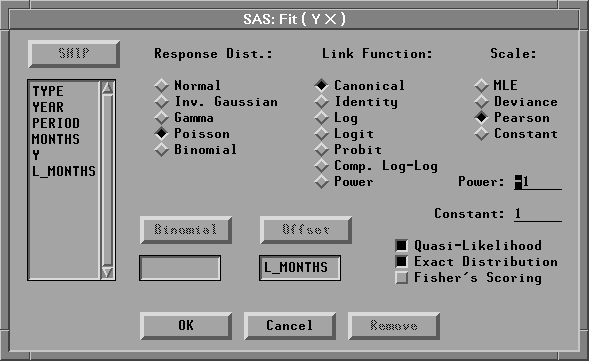
Figure 17.6: Fit Method Dialog

It is not necessary to specify a Link Function. Canonical is the default and allows

Fit ( Y X ) to choose an appropriate link. For this example, it is equivalent to choosing Log as the Link Function.

Click the OK button to close both dialogs and display the analysis.

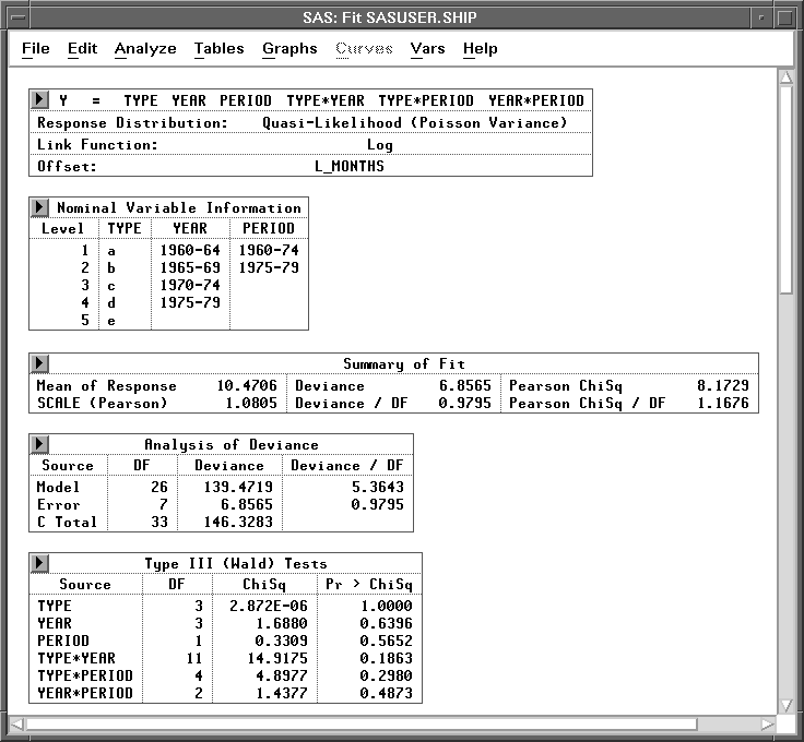
Figure 17.7: Fit Window

By default, the window includes many tables, but only a few are shown in Figure 17.7. These tables are described in the following sections. For more information about the other tables and graphs in the window, see Chapter 39, "Fit Analyses."

Note	A warning message -The negative of the Hessian is not positive definite. The convergence is questionable -appears when the specified model does not converge, as in this example. The output tables, graphs, and variables are based on the results from the last iteration.

Displaying the Poisson Regression Analysis

Model Information

Summary of Fit

Analysis of Deviance

Type III (Wald) Tests