Logistic Regression

Displaying the Logistic Regression Analysis

The PATIENT data set, described by Lee (1974), contains data collected on 27 cancer patients. The response variable, REMISS, is binary and indicates whether cancer remission occurred:

REMISS = 1 indicates success (remission occurred)

REMISS = 0 indicates failure (remission did not occur)

Several other variables containing patient characteristics thought to affect cancer remission were also included in the study. For this example, consider the following three explanatory variables: CELL, LI, and TEMP. (You may want to carry out a more complete analysis on your own.)

Open the PATIENT data set.

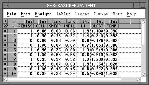
Figure 16.2: Data Window

The generalized linear model has three components:

a linear predictor function constructed from explanatory variables. For this example, the function is

$\hspace*{0.575in} {\theta}_{i} = {\beta}_{0} + {\beta}_{1} {CELL}_{i} + {\beta}_{2} {LI}_{i} + {\beta}_{3} {TEMP}_{i}$

where $\beta_0, \beta_1, \beta_2$ and ${{\beta}_{3}}$ are coefficients (parameters) for the linear predictor, and CELL_i, LI_i, and TEMP_i are the values of the explanatory variables.
a distribution or probability function for the response variable that depends on the mean ${\mu}$ and sometimes other parameters as well. For this example, the probability function is binomial.
a link function, g(.), that relates the mean to the linear predictor function. For logistic regression, the link function is the logit

$\hspace*{0.575in} g(p_{i}) = \rm{logit}(p_{i}) = {\log}(\frac{p_{i}}{1-p_{i}}) = {\theta}_{i}$

where p_i = Pr(REMISS=1 | x_i) is the response probability to be modeled, and x_i is the set of explanatory variables for the ith patient.

You can specify these three components to fit a generalized linear model by following these steps.

Choose Analyze:Fit ( Y X ) to display the fit variables dialog.

Select REMISS in the list at the left, then click the Y button.

Select CELL, LI, and TEMP in the variables list, then click the X button.

Your variables dialog should now appear, as shown in Figure 16.3.

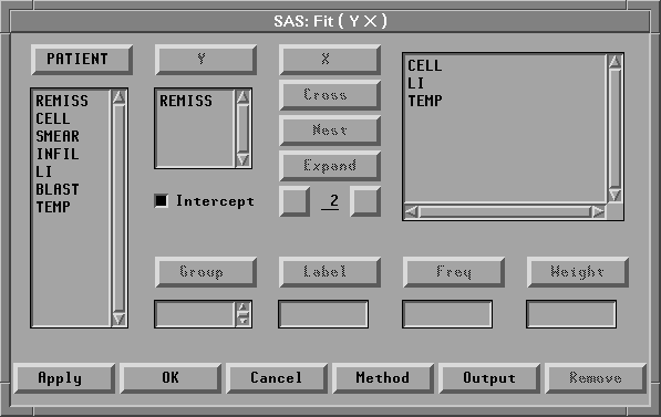
Figure 16.3: Fit Variables Dialog with Variable Roles Assigned

To specify the probability distribution for the response variable and the link function, follow these steps.

Click the Method button in the variables dialog to display the method dialog.

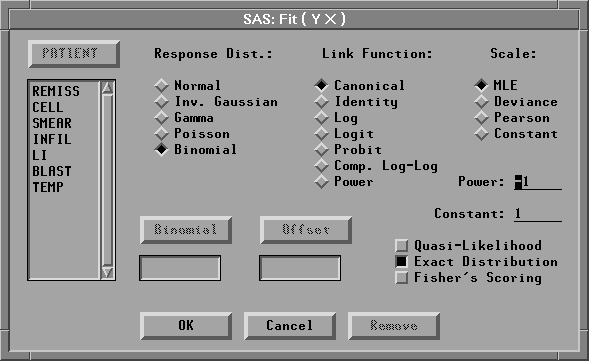
Figure 16.4: Fit Method Dialog

Click on Binomial under Response Dist to specify the probability distribution.

You do not need to specify a Link Function for this example. Canonical, the default, allows Fit ( Y X ) to choose a link dependent on the probability distribution. For the binomial distribution, as in this example, it is equivalent to choosing Logit, which yields a logistic regression.

Click the OK button to close the method dialog.

Click the Apply button in the variables dialog.

This creates the analysis shown in Figure 16.5. Recall that the Apply button causes the variables dialog to stay on the screen after the fit window appears. This is convenient for adding and deleting variables from the model.

By default, the fit window displays tables for model information, Model Equation, Summary of Fit, Analysis of Deviance, Type III (Wald) Tests, and Parameter Estimates, and a residual-by-predicted plot. You can control the tables and graphs displayed by clicking on the Output button in the fit variables dialog or by choosing from the Tables and Graphs menus.

The first table displays the model information. The first line gives the model specification. The second and third lines give the error distribution and the link function you specified in the Method dialog.

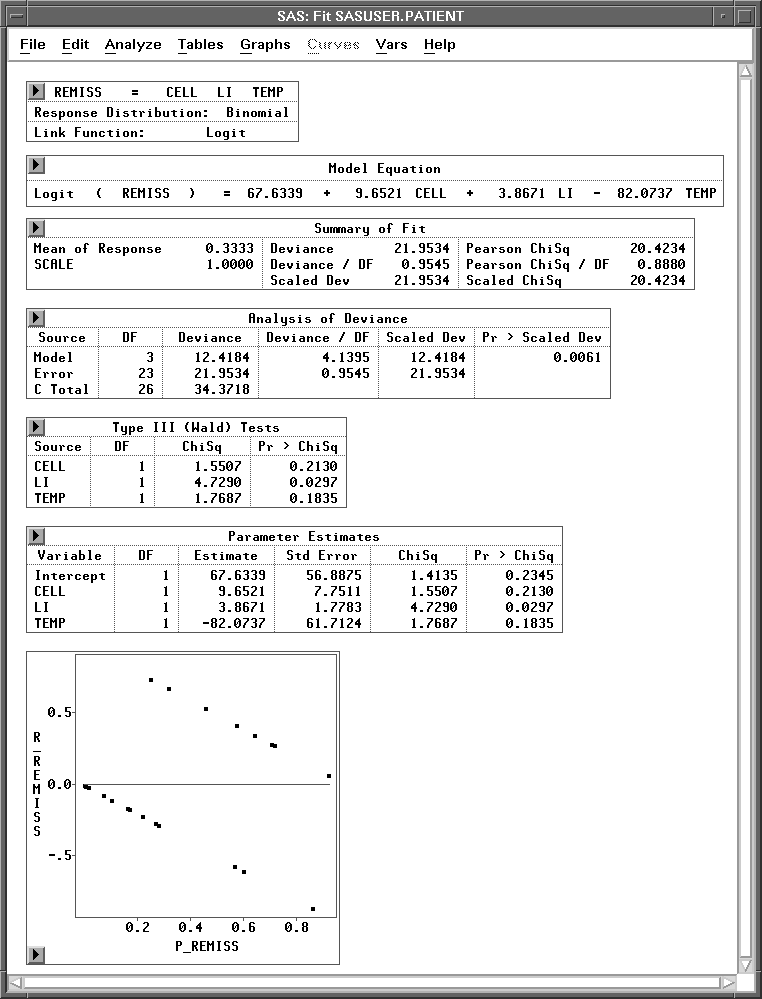
Figure 16.5: Fit Window

Displaying the Logistic Regression Analysis

Model Equation

Summary of Fit

Analysis of Deviance

Type III (Wald) Tests

Parameter Estimates Table

Residuals-by-Predicted Plot