QQ Plot

Distribution Analyses

QQ Plot

A quantile-quantile plot (QQ plot) compares ordered values of a variable with quantiles of a specific theoretical distribution. If the data are from the theoretical distribution, the points on the QQ plot lie approximately on a straight line. The normal, lognormal, exponential, and Weibull distributions can be used in the plot.

You can specify the type of QQ plot from the QQ Plot dialog after choosing Graphs:QQ Plot from the menu.

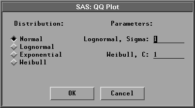
Figure 38.20: QQ Plot Dialog

In the dialog, you must specify a shape parameter for the lognormal or Weibull distribution. The normal QQ plot can also be generated with the graphs options dialog. As described later in this chapter, you can also add a reference line to the QQ plot from the Curves menu.

The following expression is used in the discussion that follows:

v_i = [(i-0.375)/(n+0.25)] for i = 1,2, ... ,n

where n is the number of nonmissing observations.

For the normal distribution, the ith ordered observation is plotted against the normal quantile $\Phi^{-1}(v_{i})$ ,where $\Phi^{-1}$ is the inverse standard cumulative normal distribution. If the data are normally distributed with mean $\mu$ and standard deviation $\sigma$ , the points on the plot should lie approximately on a straight line with intercept $\mu$ and slope $\sigma$ .The normal quantiles are stored in variables named N_name for each variable, where name is the Y variable name.

For the lognormal distribution, the ith ordered observation is plotted against the lognormal quantile $\exp(\sigma\Phi^{-1}(v_{i}))$ for a given shape parameter $\sigma$ .If the data are lognormally distributed with parameters $\theta$ , $\sigma$ , and $\zeta$ , the points on the plot should lie approximately on a straight line with intercept $\theta$ and slope $\exp(\zeta)$ .The lognormal quantiles are stored in variables named L_name for each variable, where name is the Y variable name.

For the exponential distribution, the ith ordered observation is plotted against the exponential quantile -log(1- v_i). If the data are exponentially distributed with parameters $\theta$ and $\sigma$ , the points on the plot should lie approximately on a straight line with intercept $\theta$ and slope $\sigma$ .The exponential quantiles are stored in variables named E_name for each variable, where name is the Y variable name.

For the Weibull distribution, the ith ordered observation is plotted against the Weibull quantile (-log(1- v_i))^[1/c] for a given shape parameter c. If the data are from a Weibull distribution with parameters $\theta$ , $\sigma$ , and c, the points on the plot should lie approximately on a straight line with intercept $\theta$ and slope $\sigma$ .The Weibull quantiles are stored in variables named W_name for each variable, where name is the Y variable name.

A normal QQ plot is shown in Figure 38.21. You can also add a reference line to the QQ plot from the Curves menu. You specify the intercept and slope for the reference line from the Curves menu.

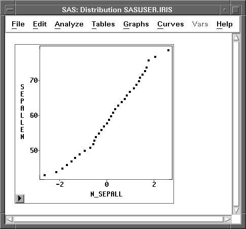
Figure 38.21: Normal QQ Plot

Further information on interpreting quantile-quantile plots can be found in Chambers et al. (1983).

If you select a Weight variable, a weighted normal QQ plot can be generated. Lognormal, exponential, and Weibull QQ plots are not computed.

For a weighted normal QQ plot, the ith ordered observation is plotted against the normal quantile $\Phi^{-1}(v_{i})$ , where

$v_{i} = \frac{(\sum_{j=1}^i{w_{(j)}}) (1-0.375/i)}{W (1+0.25/n) }$

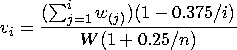
When each observation has an identical weight, w_(j)= w₀, the formulation reduces to the usual expression in the unweighted normal probability plot

v_i = [(i-0.375)/(n+0.25)]

If the data are normally distributed with mean $\mu$ and standard deviation $\sigma$ and if each observation has approximately the same weight ( w₀), then, as in the unweighted normal QQ plot, the points on the plot should lie approximately on a straight line with intercept $\mu$ and slope $\sigma$ for vardef=WDF/WGT and with slope ${\sigma/\sqrt{ w_0}}$ for vardef=DF/N.

Top of Page