PROC CAPABILITY and General Statements

Specialized Capability Indices
This section describes a number of specialized capability indices which you can request with the SPECIALINDICES option in the PROC CAPABILITY statement.
The Index k
The process capability index k (also denoted by K) is computed as
![\[ k = \frac{2 |m - \bar{X}|}{\mi{USL} - \mi{LSL}} \]](images/qcug_capability0226.png)
where 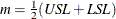 is the midpoint of the specification limits,
  is the sample mean, USL is the upper specification limit, and LSL is the lower specification limit.
The formula for k used here is given by Kane (1986). Note that k is sometimes computed without taking the absolute value of  in the numerator. See Wadsworth, Stephens, and Godfrey (1986).
If you do not specify the upper and lower limits in the SPEC statement or the SPEC= data set, then k is assigned a missing value.
Boyles’ Index 
Boyles (1992) proposed the process capability index which is defined as
![\[ C_{pm}^{+} = \frac{1}{3} { \left[ \frac{ E_{X<T} \left[ (X-T)^{2} \right] }{ (T - \mr{LSL})^{2} } + \frac{ E_{X>T} \left[ (X-T)^{2} \right] }{ (\mr{USL} - T)^{2} } \right] }^{-1/2} \]](images/qcug_capability0230.png)
He proposed this index as a modification of  for use when
  . The quantities
![\[ E_{X<T} \left[ (X-T)^{2} \right] = E \left[ (X-T)^2 | X < T \right] Pr \left[ X < T \right] \]](images/qcug_capability0232.png)
and
![\[ E_{X>T} \left[ (X-T)^{2} \right] = E \left[ (X-T)^2 | X > T \right] Pr \left[ X > T \right] \]](images/qcug_capability0233.png)
are referred to as semivariances. Kotz and Johnson (1993) point out that if  , then
  .
.
Kotz and Johnson (1993) suggest that a natural estimator for is
![\[ \widehat{C}_{pm}^{+} = \frac{1}{3} \left[ \frac{1}{n} \left\{ \frac{ \sum _{X_{i} < T} (X_{i} - T)^{2} }{ (T - \mbox{LSL})^{2} } + \frac{ \sum _{X_{i} > T} (X_{i} - T)^{2} }{ (\mbox{USL} - T)^{2} } \right\} ^{-1/2} \right] \]](images/qcug_capability0236.png)
Note that this index is not defined when either of the specification limits is equal to the target T. Refer to Section 3.5 of Kotz and Johnson (1993) for further details.
The Index 
Johnson, Kotz, and Pearn (1994) introduced a so-called "flexible" process capability index which takes into account possible differences in variability above and below the target T. They defined this index as
![\[ C_{jkp} = \frac{1}{3 \sqrt {2}} \min \left( \frac{\mbox{USL} - T}{ \sqrt { E_{X>T}[(X-T)^2] } } , \frac{T - \mbox{LSL}}{ \sqrt { E_{X<T}[(X-T)^2] } } \right) \]](images/qcug_capability0237.png)
where  .
.
A natural estimator of this index is
![\[ \widehat{C}_{jkp} = \frac{1}{3 \sqrt {2}} \min \left( \frac{ \mbox{USL} - T }{ \sqrt { \sum _{X_{i} > T} (X_{i} - T)^{2} / n } } , \frac{ T - \mbox{LSL} }{ \sqrt { \sum _{X_{i} < T} (X_{i} - T)^{2} / n } } \right) \]](images/qcug_capability0239.png)
For further details, refer to Section 4.4 of Kotz and Johnson (1993).
The Indices 
The class of capability indices , indexed by the parameter a (a > 0) allows flexibility in choosing between the relative importance of variability and deviation of the mean from the target
value T.
The class defined as
![\[ C_{pm}(a) = ( 1 - a \zeta ^2 ) C_{p} \]](images/qcug_capability0240.png)
where  . The motivation for this definition is that if
  is small, then
![\[ C_{pm} \approx (1 - \frac{1}{2} \zeta ^{2} ) C_ p \]](images/qcug_capability0243.png)
A natural estimator of is
![\[ \frac{d}{3s} \widehat{C}_{pm}(a) = \left\{ 1 - a \left( \frac{\bar{X}-T}{s} \right) ^2 \right\} \]](images/qcug_capability0244.png)
where  . You can specify the value of a with the SPECIALINDICES(CPMA=) option in the PROC CAPABILITY statement. By default, a = 0.5.
This index is not recommended for situation in which the target T is not equal to the midpoint of the specification limits.
For additional details, refer to Section 3.7 of Kotz and Johnson (1993).
The Index 
Johnson et al. (1992) suggest the class of process capability indices defined as
![\[ C_{p(\theta )} = \frac{\mbox{USL} - \mbox{LSL}}{\theta \sigma } \]](images/qcug_capability0246.png)
where  is chosen so that the proportion of conforming items is robust with respect to the shape of the process distribution. In
particular, Kotz and Johnson (1993) recommend use of
is chosen so that the proportion of conforming items is robust with respect to the shape of the process distribution. In
particular, Kotz and Johnson (1993) recommend use of
![\[ C_{p(5.15)} = \frac{\mbox{USL} - \mbox{LSL}}{5.15 \sigma } \]](images/qcug_capability0248.png)
which is estimated as
![\[ \widehat{C}_{p(5.15)} = \frac{\mbox{USL} - \mbox{LSL}}{5.15 s} \]](images/qcug_capability0249.png)
For details, refer to Section 4.3.2 of Kotz and Johnson (1993).
The Index 
Similarly, Kotz and Johnson (1993) recommend use of the robust capability index
![\[ C_{pk(5.15)} = \frac{d - | \mu - (\mbox{USL} + \mbox{LSL}) / 2 | }{2.575 \sigma } \]](images/qcug_capability0251.png)
where . This index is estimated as
![\[ \widehat{C}_{pk(5.15)} = \frac{d - | \bar{X} - (\mbox{USL} + \mbox{LSL}) / 2 |}{2.575 s} \]](images/qcug_capability0252.png)
For details, refer to Section 4.3.2 of Kotz and Johnson (1993).
The Index 
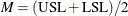
Pearn, Kotz, and Johnson (1992) proposed the index
![\[ C_{pmk} = \frac{(\mbox{USL} - \mbox{LSL})/2 - |\mu - m |}{3 \sqrt { \sigma ^2 + (\mu - T)^2}} \]](images/qcug_capability0253.png)
where  . A natural estimator for is
![\[ \widehat{C}_{pmk} = \frac{(\mbox{USL} - \mbox{LSL})/2 - |\bar{X} - m |}{3 \sqrt {(\frac{n-1}{n})s^2 + (\bar{X} - T)^2}} \]](images/qcug_capability0255.png)
where 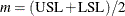 .
.
For further details, refer to Section 3.6 of Kotz and Johnson (1993).
Wright’s Index 
Wright (1995) defines the capability index
![\[ C_ s = \frac{ \min \left( \mr{USL} - \mu , \mu - \mr{LSL} \right) }{ 3 \sqrt { \sigma ^2 + (\mu - T)^2 + \mu _3 / \sigma } } \]](images/qcug_capability0256.png)
where  .
.
A natural estimator of  is
is
![\[ \widehat{C}_ s = \frac{ ( \mr{USL} - \mr{LSL} ) / 2 - | \bar{X} - m | }{ 3 \sqrt { \left( \frac{n-1}{n} \right) s^2 + (\bar{X} - T)^2 + |c_4 s^2 b_3| } } \]](images/qcug_capability0258.png)
where  is an unbiasing constant for the sample standard deviation, and
  is a measure of skewness. Wright (1995) shows that compares favorably with even when skewness is not present, and he advocates the use of for monitoring near-normal processes when loss of capability typically leads to asymmetry.
Chen and Kotz (1996) proposed a modification to Wright’s index which introduces a multiplier,  , and is estimated as
![\[ \widehat{C}_ s = \frac{ ( \mr{USL} - \mr{LSL} ) / 2 - | \bar{X} - m | }{ 3 \sqrt { \left( \frac{n-1}{n} \right) s^2 + (\bar{X} - T)^2 + \gamma |c_4 s^2 b_3| } } \]](images/qcug_capability0262.png)
If you specify a value for  with the SPECIALINDICES(CSGAMMA=) option, the index is computed with this modification. Otherwise it is computed using Wright’s original definition.
The Index 
Boyles (1994) proposed a smooth version of defined as
![\[ S_{jkp} = S \left( \frac{\mbox{USL} - T}{ \sqrt { 2 E_{X>T}[(X-T)^2] } } , \frac{T - \mbox{LSL}}{ \sqrt { 2 E_{X<T}[(X-T)^2] } } \right) \]](images/qcug_capability0263.png)
The CAPABILITY procedure estimates as
![\[ \widehat{S}_{jkp} = S \left( \frac{ \mbox{USL} - T }{ \sqrt { 2 \sum _{X_{i} > T} (X_{i} - T)^{2} / n } } , \frac{ T - \mbox{LSL} }{ \sqrt { 2 \sum _{X_{i} < T} (X_{i} - T)^{2} / n } } \right) \]](images/qcug_capability0264.png)
where ![$S(x,y) = \Phi ^{-1}[\{ \Phi (x) + \Phi (y)\} /2]/3$](images/qcug_capability0265.png) .
.
The Index 
Chen (1998) devised a process incapability index based on the  index. The first term measures inaccuracy and the second measures imprecision. The index is estimated as
![\[ \widehat{C}_{pp} = \left( \frac{~ \bar{X} - T}{d^{*} / 3} \right)^2 + \left( \frac{s}{d^{*} / 3} \right)^2 \]](images/qcug_capability0267.png)
where  .
.
The Index 
The index does not handle asymmetric tolerances well, as discussed by Kotz and Lovelace (1998). To address that shortcoming, Chen (1998) defined the index , which is estimated by
![\[ \widehat{C}_{pp}^{''} = \left( \frac{\widehat{A}}{d^{*} / 3} \right)^2 + \left( \frac{s}{d^{*} / 3} \right) \]](images/qcug_capability0269.png)
where
![\[ \widehat{A} = \max \left\{ \frac{(\bar{X} - T)d}{T - \mbox{LSL}} , \frac{(T - \bar{X})d}{\mbox{USL} - T} \right\} \]](images/qcug_capability0270.png)
and 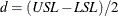 .
.

![\[ C_{pg} = \frac{1}{C_{pm}^2} \]](images/qcug_capability0272.png)
![\[ \widehat{C}_{pg} = \frac{1}{\widehat{C}_{pm}^2} \]](images/qcug_capability0273.png)

![\[ \widehat{C}_{pq} = \widehat{C}_ p \left[ 1 - \frac{1}{2} \left( \frac{\bar{X} - T}{s} \right)^2 \right] \]](images/qcug_capability0274.png)
The Index 
Bai and Choi (1997) defined the index
![\[ C_ p^ W = \frac{C_ p}{\sqrt { 1 + | 1 - 2 P_ x | }} \]](images/qcug_capability0276.png)
where  . It is estimated by
![\[ \widehat{C}_ p^ W = \frac{\widehat{C}_ p}{\sqrt { 1 + | 1 - 2 \widehat{P}_ x | }} \]](images/qcug_capability0278.png)
where  is the fraction of observations less than or equal to . For more information about , see Kotz and Lovelace (1998).
The Index 
Bai and Choi (1997) also proposed the index
![\[ C_{pk}^ W = \min \left\{ \frac{\mbox{USL} - \mu }{3 \sigma \sqrt {2 P_ x}} , \frac{\mu - \mbox{LSL}}{3 \sigma \sqrt {2 (1 - P_ x)}} \right\} \]](images/qcug_capability0281.png)
It is estimated by
![\[ \widehat{C}_{pk}^ W = \min \left\{ \frac{\mbox{USL} - \bar{X}}{3 s \sqrt {2 \widehat{P}_ x}} , \frac{\bar{X} - \mbox{LSL}}{3 s \sqrt {2 (1 - \widehat{P}_ x)}} \right\} \]](images/qcug_capability0282.png)
where is the fraction of observations less than or equal to . For more information about , see Kotz and Lovelace (1998).
The Index 
The index , also introduced by Bai and Choi (1997), is defined as
![\[ C_{pm}^ W = \frac{C_{pm}}{\sqrt {1 + | 1 - 2P_ T |}} \]](images/qcug_capability0283.png)
where  . It is estimated by
![\[ \widehat{C}_{pm}^ W = \frac{\widehat{C}_{pm}}{\sqrt {1 + | 1 - 2 \widehat{P}_ T | }} \]](images/qcug_capability0285.png)
where  is the fraction of observations less than or equal to T. For more information about
  , see Kotz and Lovelace (1998).

![\[ C_{pc} = \frac{\mbox{USL} - \mbox{LSL}}{6 \sqrt {\frac{\pi }{2} E |X - M|}} \]](images/qcug_capability0288.png)
![\[ \widehat{C}_{pc} = \frac{\mbox{USL} - \mbox{LSL}}{6 \sqrt {\frac{\pi }{2} c}} \]](images/qcug_capability0290.png)
![\[ c = \frac{1}{n} \sum _{i = 1}^ n | X_ i - M | \]](images/qcug_capability0291.png)
Vännmann’s Index 
Vännmann (1995) introduced the generalized index , which reduces to the following capability indices given appropriate choices of u and v:


is defined as
![\[ C_ p(u,v) = \frac{d - u |~ \mu - M|}{3 \sqrt {\sigma ^2 + v(~ \mu - T)^2}} \]](images/qcug_capability0296.png)
and estimated by
![\[ \widehat{C}_ p(u,v) = \frac{d - u |\bar{X} - M|}{3 \sqrt {(\frac{n - 1}{n})s^2 + v(\bar{X} - T)^2}} \]](images/qcug_capability0297.png)
You can specify u with the SPECIALINDICES(CPU=) option and v with the SPECIALINDICES(CPV=) option. By default, u = 0 and v = 4.
Vännmann’s Index 
Vännmann (1997) also proposed the index , which is equivalent to  with u = 1. It is estimated as
![\[ \widehat{C}_ p(v) = \frac{d - |\bar{X} - M|}{3 \sqrt {(\frac{n - 1}{n})s^2 + v(\bar{X} - T)^2}} \]](images/qcug_capability0299.png)
You can specify v with the SPECIALINDICES(CPV=) option. By default, v = 4.