Example 5.12 Computing Kernel Density Estimates

Note: See Superimposing Kernel Density Estimates in the SAS/QC Sample Library.

This example illustrates the use of kernel density estimates to visualize a nonnormal data distribution.

The effective channel length (in microns) is measured for 1225 field effect transistors. The channel lengths are saved as values of the variable Length in a SAS data set named Channel:

data Channel;
   length Lot $ 16;
   input Length @@;
   select;
      when (_n_ <= 425) Lot='Lot 1';
      when (_n_ >= 926) Lot='Lot 3';
      otherwise Lot='Lot 2';
   end;
   datalines;
0.91 1.01 0.95 1.13 1.12 0.86 0.96 1.17 1.36 1.10
0.98 1.27 1.13 0.92 1.15 1.26 1.14 0.88 1.03 1.00
0.98 0.94 1.09 0.92 1.10 0.95 1.05 1.05 1.11 1.15
1.11 0.98 0.78 1.09 0.94 1.05 0.89 1.16 0.88 1.19
1.01 1.08 1.19 0.94 0.92 1.27 0.90 0.88 1.38 1.02

   ... more lines ...   

1.80 2.35 2.23 1.96 2.16 2.08 2.06 2.03 2.18 1.83
2.13 2.05 1.90 2.07 2.15 1.96 2.15 1.89 2.15 2.04
1.95 1.93 2.22 1.74 1.91
;

When you use kernel density estimates to explore a data distribution, you should try several choices for the bandwidth parameter c because this determines the smoothness and closeness of the fit. You can specify a list of C= values with the KERNEL option to request multiple density estimates, as shown in the following statements:

title "FET Channel Length Analysis";
proc capability data=Channel noprint;
   histogram Length / kernel(c = 0.25 0.50 0.75 1.00)
                      odstitle = title;
run;

The display, shown in Output 5.12.1, demonstrates the effect of c. In general, larger values of c yield smoother density estimates, and smaller values yield estimates that more closely fit the data distribution.

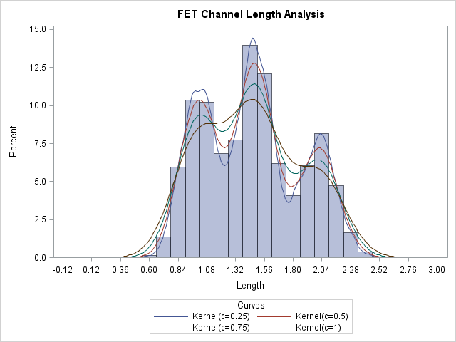
Output 5.12.1: Multiple Kernel Density Estimates

Output 5.12.1 reveals strong trimodality in the data, which are explored further in Creating a One-Way Comparative Histogram.

HISTOGRAM Statement: CAPABILITY Procedure

Example 5.12 Computing Kernel Density Estimates