Adding a Normal Curve to the Histogram :: SAS/QC(R) 13.1 User's Guide

Adding a Normal Curve to the Histogram

Note: See Histogram with Fitted Normal Curve in the SAS/QC Sample Library.

This example is a continuation of the preceding example.

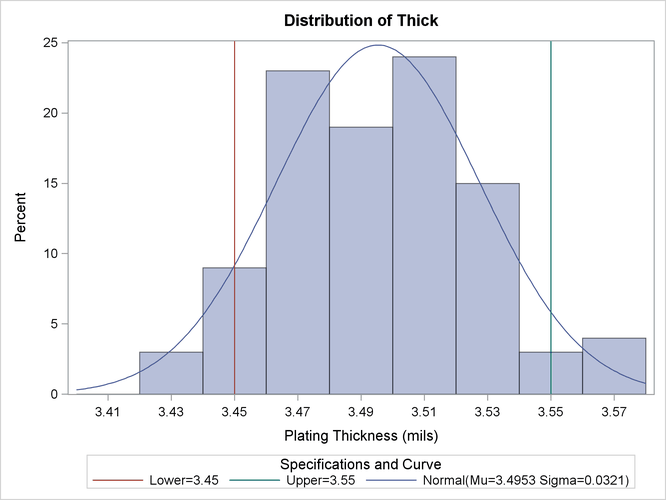
The following statements fit a normal distribution from the thickness measurements and superimpose the fitted density curve on the histogram:

proc capability data=Trans;
   spec lsl = 3.45 usl = 3.55;
   histogram / normal;
run;

The ODS GRAPHICS ON statement specified before the PROC CAPABILITY statement enables ODS Graphics, so the histogram is created using ODS Graphics instead of traditional graphics.

The NORMAL option summarizes the fitted distribution in the printed output shown in Figure 5.9, and it specifies that the normal curve be displayed on the histogram shown in Figure 5.10.

Figure 5.9: Summary for Fitted Normal Distribution

Process Capability Analysis of Plating Thickness

The CAPABILITY Procedure

Fitted Normal Distribution for Thick (Plating Thickness (mils))

Parameters for Normal Distribution
Parameter	Symbol	Estimate
Mean	Mu	3.49533
Std Dev	Sigma	0.032117

Goodness-of-Fit Tests for Normal Distribution
Test	Statistic		DF	p Value
Kolmogorov-Smirnov	D	0.05563823		Pr > D	>0.150
Cramer-von Mises	W-Sq	0.04307548		Pr > W-Sq	>0.250
Anderson-Darling	A-Sq	0.27840748		Pr > A-Sq	>0.250
Chi-Square	Chi-Sq	6.96953022	5	Pr > Chi-Sq	0.223

Percent Outside Specifications for Normal Distribution
Lower Limit		Upper Limit
LSL	3.450000	USL	3.550000
Obs Pct < LSL	8.000000	Obs Pct > USL	5.000000
Est Pct < LSL	7.906248	Est Pct > USL	4.435722

Quantiles for Normal Distribution
Percent	Quantile
Percent	Observed	Estimated
1.0	3.42950	3.42061
5.0	3.44300	3.44250
10.0	3.45750	3.45417
25.0	3.46950	3.47367
50.0	3.49600	3.49533
75.0	3.51650	3.51699
90.0	3.53550	3.53649
95.0	3.55300	3.54816
99.0	3.57200	3.57005

Figure 5.10: Histogram Superimposed with Normal Curve

The printed output includes the following:

parameters for the normal curve. The normal parameters $\mu$ and $\sigma$ are estimated by the sample mean ( $\hat{\mu }=3.49533$ ) and the sample standard deviation ( $\hat{\sigma }=0.032117$ ).
goodness-of-fit tests based on the empirical distribution function (EDF): the Anderson-Darling, Cramer-von Mises, and Kolmogorov-Smirnov tests. The p-values for these tests are greater than the usual cutoff values of 0.05 and 0.10, indicating that the thicknesses are normally distributed.
a chi-square goodness-of-fit test. The p-value of 0.223 for this test indicates that the thicknesses are normally distributed. In general EDF tests (when available) are preferable to chi-square tests. See the section EDF Goodness-of-Fit Tests for details.
observed and estimated percentages outside the specification limits
observed and estimated quantiles

For details, including formulas for the goodness-of-fit tests, see Printed Output. Note that the NOPRINT option in the PROC CAPABILITY statement suppresses only the printed output with summary statistics for the variable Thick. To suppress the printed output in Figure 5.9, specify the NOPRINT option enclosed in parentheses after the NORMAL option as in Customizing a Histogram.

The NORMAL option is one of many options that you can specify in the HISTOGRAM statement. See the section Syntax: HISTOGRAM Statement for a complete list of options or the section Dictionary of Options for detailed descriptions of options.

HISTOGRAM Statement: CAPABILITY Procedure

Adding a Normal Curve to the Histogram