Example 17.26 OC Curve for Chart :: SAS/QC(R) 12.3 User's Guide

Example 17.26 OC Curve for Chart

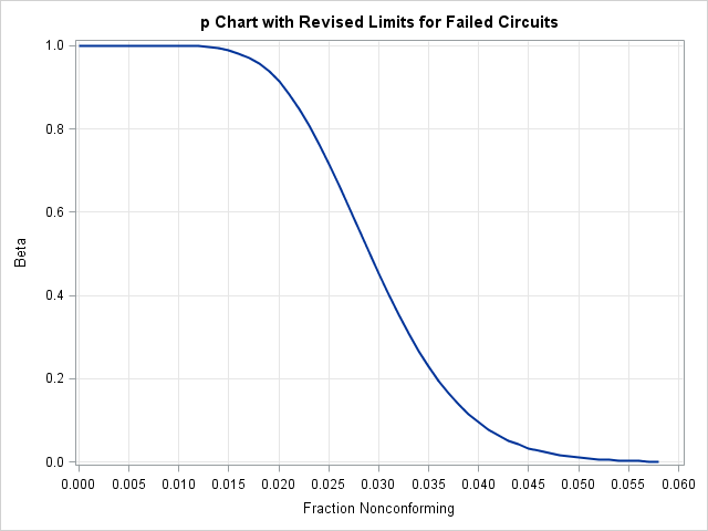
See SHWPOC in the SAS/QC Sample LibraryThis example uses the GPLOT procedure and the OUTLIMITS= data set Faillim2 from the previous example to plot an OC curve for the p chart shown in Output 17.25.3.

The OC curve displays $\beta$ (the probability that lies within the control limits) as a function of p (the true proportion nonconforming). The computations are exact, assuming that the process is in control and that the number of nonconforming items () has a binomial distribution.

The value of $\beta$ is computed as follows:

$\displaystyle \beta$	$\displaystyle =$	$\displaystyle P(p_{i} \leq \mbox{UCL}) - P(p_{i} < \mbox{LCL})$
$\displaystyle$	$\displaystyle =$	$\displaystyle P(X_{i} \leq n \mbox{UCL}) - P(X_{i} < n \mbox{LCL})$
$\displaystyle$	$\displaystyle =$	$\displaystyle P(X_{i} < n\mbox{UCL}) + P(X_{i} = n\mbox{UCL}) - P(X_{i} < n\mbox{LCL})$
$\displaystyle$	$\displaystyle =$	$\displaystyle I_{1-p} (n + 1 - n \mbox{UCL},n\mbox{UCL})+ P(X_{i} = n\mbox{UCL})- I_{1-p} (n + 1 - n\mbox{LCL}, n\mbox{LCL})$
$\displaystyle$	$\displaystyle =$	$\displaystyle I_{p} (n\mbox{LCL}, n + 1 - n\mbox{LCL})+ P(X_{i} = n\mbox{UCL}) - I_{p} (n\mbox{UCL}, n + 1 - n\mbox{UCL})$

Here, $I_ p(\cdot , \cdot )$ denotes the incomplete beta function. The following DATA step computes $\beta$ (the variable BETA) as a function of p (the variable P):

data ocpchart;
   set Faillim2;
   keep beta fraction _lclp_ _p_ _uclp_;
   nucl=_limitn_*_uclp_;
   nlcl=_limitn_*_lclp_;
   do p=0 to 500;
      fraction=p/1000;
      if nucl=floor(nucl) then
         adjust=probbnml(fraction,_limitn_,nucl) -
                probbnml(fraction,_limitn_,nucl-1);
      else adjust=0;
      if nlcl=0 then
         beta=1 - probbeta(fraction,nucl,_limitn_-nucl+1) + adjust;
      else beta=probbeta(fraction,nlcl,_limitn_-nlcl+1) -
                probbeta(fraction,nucl,_limitn_-nucl+1) +
                adjust;
      if beta >= 0.001 then output;
   end;
   call symput('lcl', put(_lclp_,5.3));
   call symput('mean',put(_p_,   5.3));
   call symput('ucl', put(_uclp_,5.3));
run;

The following statements display the OC curve shown in Output 17.26.1:

proc sgplot data=ocpchart;
   series x=fraction y=beta / lineattrs=(thickness=2);
   xaxis values=(0 to 0.06 by 0.005) grid;
   yaxis grid;
   label fraction = 'Fraction Nonconforming'
         beta     = 'Beta';
run;

Output 17.26.1: OC Curve for p Chart

PCHART Statement: SHEWHART Procedure

Example 17.26 OC Curve for Chart