BOXCHART Statement: SHEWHART Procedure

Constructing Box Charts

The following notation is used in this section:

$\mu$	process mean (expected value of the population of measurements)
$\sigma$	process standard deviation (standard deviation of the population of measurements)
$\bar{X}_{i}$	mean of measurements in ith subgroup
$n_{i}$	sample size of ith subgroup
N	the number of subgroups
$x_{ij}$	jth measurement in the ith subgroup, $j=1,2,3 \ldots , n_{i}$
$x_{i(j)}$	jth largest measurement in the ith subgroup: $x_{i(1)} \leq x_{i(2)} \leq \ldots \leq x_{i(n_{i})}$
$\overline{\overline{X}}$	weighted average of subgroup means
$M_{i}$	median of the measurements in the ith subgroup: $M_ i = \left\{ \begin{array}{ll} x_{i((n_ i + 1)/2)} & \mbox{if $n_{i}$ is odd} \\ (x_{i(n_ i/2)} + x_{i((n_ i/2)+1)})/2 & \mbox{if $n_{i}$ is even} \end{array} \right.$
$\bar{M}$	average of the subgroup medians: $\bar{M} = (n_1M_1 + \ldots + n_ NM_ N)/(n_1+\ldots +n_ N)$
$\tilde{M}$	median of the subgroup medians. Denote the jth largest median by $M_{(j)}$ so that $M_{(1)} \leq M_{(2)}\leq \ldots \leq M_{(N)}$ . $\tilde{M} = \left\{ \begin{array}{ll} M_{((N+1)/2)} & \mbox{if \Mathtext{N} is odd} \\ (M_{(N/2)} + M_{(N/2)+1})/2 & \mbox{if \Mathtext{N} is even} \end{array} \right.$
	standard error of the median of n independent, normally distributed variables with unit standard deviation (the value of can be calculated with the STDMED function in a DATA step)
$Q_{p}(n)$	$100 \times p$ th percentile (0 < p < 1) of the distribution of the median of n independent observations from a normal population with unit standard deviation
$z_{p}$	$100 \times p$ th percentile of the standard normal distribution
$D_{p}(n)$	$100 \times p$ th percentile of the distribution of the range of n independent observations from a normal population with unit standard deviation

Elements of Box-and-Whisker Plots

A box-and-whisker plot is displayed for the measurements in each subgroup on the box chart. Figure 17.14 illustrates the elements of each plot.

Figure 17.14: Box-and-Whisker Plot

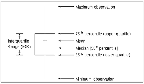
The skeletal style of the box-and-whisker plot shown in Figure 17.14 is the default. You can specify alternative styles with the BOXSTYLE= option; see Example 17.2 or the entry for BOXSTYLE= in Dictionary of Options: SHEWHART Procedure.

Control Limits and Central Line

You can compute the limits in the following ways:

as a specified multiple (k) of the standard error of $\bar{X}_{i}$ (or $M_{i}$ ) above and below the central line. The default limits are computed with k = 3 (these are referred to as $3\sigma$ limits).
as probability limits defined in terms of $\alpha$ , a specified probability that $\bar{X}_{i}$ (or $M_{i}$ ) exceeds the limits

The CONTROLSTAT= option specifies whether control limits are computed for subgroup means (the default) or subgroup medians. The following tables provide the formulas for the limits:

Table 17.5: Control Limits and Central Line for Box Charts

CONTROLSTAT=MEAN	CONTROLSTAT=MEDIAN
LCLX = lower limit = $\overline{\overline{X}} - k\hat{\sigma }/ \sqrt {n_{i}}$	LCLM = lower limit = $\bar{M} - k\hat{\sigma }e_{M}(n_ i)$
Central Line = $\overline{\overline{X}}$	Central Line = $\bar{M}$
UCLX = upper limit = $\overline{\overline{X}} + k\hat{\sigma }/ \sqrt {n_{i}}$	UCLM = upper limit = $\bar{M} + k\hat{\sigma }e_{M}(n_ i)$

Table 17.6: Probability Limits and Central Line for Box Charts

CONTROLSTAT=MEAN	CONTROLSTAT=MEDIAN
LCLX = lower limit = $\overline{\overline{X}} - z_{\alpha /2}(\hat{\sigma }/ \sqrt {n_{i}})$	LCLM = lower limit = $\bar{M} - Q_{\alpha /2}(n_ i)\hat{\sigma }$
Central Line = $\overline{\overline{X}}$	Central Line = $\bar{M}$
UCLX = upper limit = $\overline{\overline{X}} + z_{\alpha /2}(\hat{\sigma }/ \sqrt {n_{i}})$	UCLM = upper limit = $\bar{M} + Q_{1-\alpha /2}(n_ i)\hat{\sigma }$

In the preceding tables, replace $\bar{M}$ with $\overline{\overline{X}}$ if you specify MEDCENTRAL=AVGMEAN in addition to CONTROLSTAT=MEDIAN. Likewise, replace $\bar{M}$ with $\tilde{M}$ if you specify MEDCENTRAL=MEDMED in addition to CONTROLSTAT=MEDIAN. If standard values $\mu _{0}$ and $\sigma _{0}$ are available for $\mu$ and $\sigma$ , replace $\overline{\overline{X}}$ with $\mu _{0}$ and $\hat{\sigma }$ with $\sigma _{0}$ in Table 17.5 and Table 17.6.

Note that the limits vary with $n_{i}$ . The formulas for median limits assume that the data are normally distributed.

You can specify parameters for the limits as follows:

Specify k with the SIGMAS= option or with the variable _SIGMAS_ in a LIMITS= data set.
Specify $\alpha$ with the ALPHA= option or with the variable _ALPHA_ in a LIMITS= data set.
Specify a constant nominal sample size $n_{i} \equiv n$ for the control limits with the LIMITN= option or with the variable _LIMITN_ in a LIMITS= data set.
Specify $\mu _{0}$ with the MU0= option or with the variable _MEAN_ in a LIMITS= data set.
Specify $\sigma _{0}$ with the SIGMA0= option or with the variable _STDDEV_ in a LIMITS= data set.

Note: You can suppress the display of the control limits with the NOLIMITS option. This is useful for creating standard side-by-side box-and-whisker plots.