Determining the Components of Variation
The standard Shewhart analysis assumes that sampling variation, also referred to as within-group variation, is the only source of variation. Writing  for the
  th measurement within the
  th subgroup, you can express the model for the conventional
  and
and  chart as
 |
for  and
and  . The random variables
  are assumed to be independent with zero mean and unit variance, and
  is the within-subgroup variance. The parameter
  denotes the process mean.
In a process such as film manufacturing, this model is not adequate because there is additional variation due to changes in temperature, pressure, raw material, and other factors. A more appropriate model is
 |
where  is the between-subgroup variance, the random variables
  are independent with zero mean and unit variance, and the random variables are independent of the random variables .1
To plot the subgroup averages  on a control chart, you need expressions for the expectation and variance of
  . These are
 |
Thus, the central line should be located at  , and
, and  limits should be located at
 |
where  and
and  denote estimates of the variance components. You can use a variety of SAS procedures for fitting linear models to estimate the variance components. The following statements show how this can be done with the MIXED procedure:
title;
proc mixed data=Film2;
   class Sample;
   model Testval = / s;
   random Sample;
   ods output solutionf=sf;
   ods output covparms=cp;
run;
The results are shown in Figure 15.203. Note that the parameter estimates are  ,
,  , and
, and  .
.
| Covariance Parameter Estimates | |
|---|---|
| Cov Parm | Estimate |
| Sample | 19.2526 |
| Residual | 39.6825 |
| Solution for Fixed Effects | |||||
|---|---|---|---|---|---|
| Effect | Estimate | Standard Error | DF | t Value | Pr > |t| |
| Intercept | 88.8963 | 0.7250 | 55 | 122.61 | <.0001 |
The following statements merge the output data sets from the MIXED procedure into a SAS data set named Newlim that contains the appropriately derived control limit parameters for average test value:
data cp;
   set cp sf;
   keep Estimate;
run;

proc transpose data=cp out=Newlim;
run;

data Newlim (keep=_lclx_ _mean_ _uclx_);
  set Newlim;
  _limitn_ = 4;
  _mean_   = col3;
  _stddev_ = sqrt(4*col1 + col2);
  _lclx_   = _mean_ - 3*_stddev_ / sqrt(_limitn_);
  _uclx_   = _mean_ + 3*_stddev_ / sqrt(_limitn_);
  output;
run;
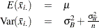
Here, the variable _LIMITN_ is assigned the value of  , the variable _MEAN_ is assigned the value of , and the variable _STDDEV_ is assigned the value of
 |
The limits (_LCLX_ and _UCLX_) are computed according to (3) using  . The data set Newlim contains the mean and limits for the average test value.
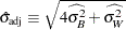
The following statements compute appropriate control limits for the and charts, which are shown in Figure 15.204. First, the data set Newlim2 is created by merging the data set RLimits, which contains the original chart limits computed in Preliminary Examination of Variation, with Newlim, which saved the appropriate chart limits. The original chart limits are valid because the range in the th subgroup is  , which is the same for models (1) and (2). The LIMITS= option specifies the data set Newlim2 as the source of the control limits for Figure 15.204.
data Newlim2;
   merge Newlim RLimits (drop=_lclx_ _mean_ _uclx_);
run;

title 'Control Chart with Adjusted Limits';
symbol h = 2.0 pct;
proc shewhart data=Film2 limits=Newlim2;
   xrchart Testval*Sample / npanelpos = 60;
   label Testval='Average Test Value';
run;
The control limits for the chart in Figure 15.204 are  . This chart correctly indicates that the variation in the process is due to common causes.
and Chart with Derived Control Limits
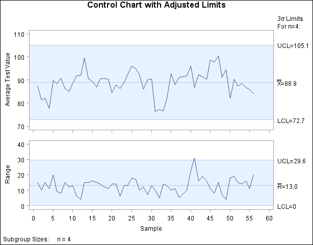
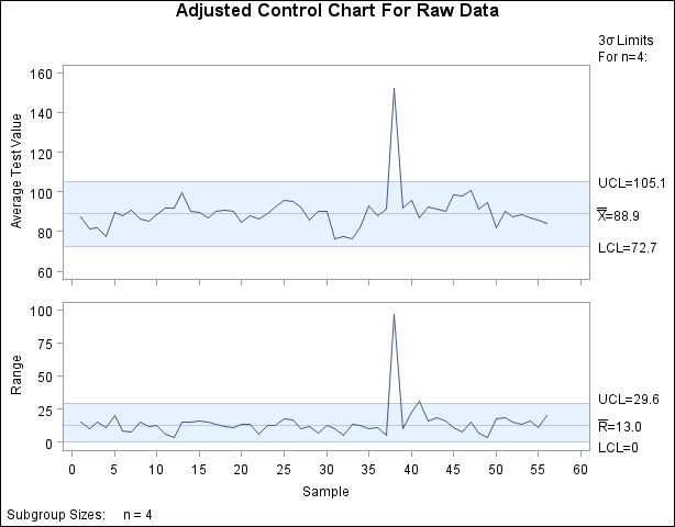
You can use a similar set of statements to display the derived control limits in Newlim on an and chart for the original data (including outliers), as shown in Figure 15.205.
and Chart with Derived Control Limits for Raw Data
A simple alternative to the chart in Figure 15.204 is an "individual measurements" chart for the subgroup means. The advantage of the variance components approach is that it yields separate estimates of the components due to lane and sample, as well as a number of hypothesis tests (these require assumptions of normality). In applying this method, however, you should be careful to use data that represent the process in a state of statistical control.
Footnotes
- This notation is used in Chapter 3 of Wetherill and Brown (1991), which discusses this issue.