XCHART Statement: SHEWHART Procedure

Plotted Points

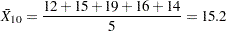
Each point on an chart indicates the value of a subgroup mean (). For example, if the tenth subgroup contains the values 12, 15, 19, 16, and 14, the value plotted for this subgroup is

Central Line

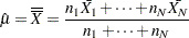
By default, the central line on an chart indicates an estimate for , which is computed as

If you specify a known value () for , the central line indicates the value of .

Control Limits

You can compute the limits in the following ways:

• as a specified multiple () of the standard error of above and below the central line. The default limits are computed with (these are referred to as limits).

• as probability limits defined in terms of , a specified probability that exceeds the limits

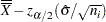
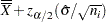
The following table provides the formulas for the limits:

Table 15.65 Limits for Charts

Control Limits
LCL lower limit =
UCL upper limit =

Note that the limits vary with . If standard values and are available for and , respectively, replace with and with in Table 15.65.

You can specify parameters for the limits as follows:

• Specify with the SIGMAS= option or with the variable _SIGMAS_ in a LIMITS= data set.

• Specify with the ALPHA= option or with the variable _ALPHA_ in a LIMITS= data set.

• Specify a constant nominal sample size for the control limits with the LIMITN= option or with the variable _LIMITN_ in a LIMITS= data set.

• Specify with the MU0= option or with the variable _MEAN_ in a LIMITS= data set.

• Specify with the SIGMA0= option or with the variable _STDDEV_ in a LIMITS= data set.