SCHART Statement: SHEWHART Procedure

Reading Preestablished Control Limits

[See SHWSCHR in the SAS/QC Sample Library]In the previous example, the OUTLIMITS= data set Turblim saved control limits computed from the measurements in Turbine. This example shows how these limits can be applied to new data.

The following statements create an chart for new measurements in the data set Turbine2 (not listed here) using the control limits in Turblim:

ods graphics on;
title 'Chart for Standard Deviations of Power Output';
proc shewhart data=Turbine2 limits=Turblim;
   schart KWatts*Day / odstitle=title;
run;

The ODS GRAPHICS ON statement specified before the PROC SHEWHART statement enables ODS Graphics, so the chart is created by using ODS Graphics instead of traditional graphics. The chart is shown in Figure 15.86.

The LIMITS= option in the PROC SHEWHART statement specifies the data set containing the control limits. By default,¹ this information is read from the first observation in the LIMITS= data set for which

• the value of _VAR_ matches the process name KWatts

• the value of _SUBGRP_ matches the subgroup-variable name Day

Figure 15.86 Chart for Second Set of Power Output Data (ODS Graphics)

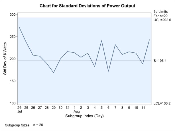
All the standard deviations lie within the control limits, indicating that the variability of the heating process is still in statistical control.

In this example, the LIMITS= data set was created in a previous run of the SHEWHART procedure. You can also create a LIMITS= data set with the DATA step. See LIMITS= Data Set for details concerning the variables that you must provide.