RCHART Statement: SHEWHART Procedure

Creating Range Charts from Summary Data
[See SHWRCHR in the SAS/QC Sample Library]The previous example illustrates how you can create  charts using raw data (process measurements). However, in many applications the data are provided as subgroup summary statistics. This example illustrates how you can use the RCHART statement with data of this type.
The following data set (Disksum) provides the data from the preceding example in summarized form:
data Disksum;
   input Lot TimeX TimeR;
   TimeN=6;
datalines;
  1  8.00833  0.16
  2  8.02167  0.09
  3  7.97833  0.07
  4  8.00667  0.10
  5  8.01833  0.16
  6  8.00667  0.12
  7  7.98500  0.15
  8  8.03000  0.11
  9  8.03000  0.15
 10  7.99167  0.10
 11  7.98833  0.10
 12  7.98500  0.09
 13  7.98833  0.13
 14  8.00167  0.10
 15  7.98333  0.13
 16  8.01833  0.09
 17  8.00833  0.11
 18  7.98667  0.20
 19  7.98667  0.18
 20  8.01500  0.10
 21  7.99000  0.14
 22  8.01833  0.20
 23  8.00833  0.11
 24  7.98500  0.06
 25  8.03667  0.15
;
A partial listing of Disksum is shown in Figure 15.73. There is exactly one observation for each subgroup (note that the subgroups are still indexed by Lot). The variable TimeX contains the subgroup means, the variable TimeR contains the subgroup ranges, and the variable TimeN contains the subgroup sample sizes (these are all six).
| The Summary Data Set of Disk Drive Test Times |
| Lot | TimeX | TimeR | TimeN |
|---|---|---|---|
| 1 | 8.00833 | 0.16 | 6 |
| 2 | 8.02167 | 0.09 | 6 |
| 3 | 7.97833 | 0.07 | 6 |
| 4 | 8.00667 | 0.10 | 6 |
| 5 | 8.01833 | 0.16 | 6 |
You can read this data set by specifying it as a HISTORY= data set in the PROC SHEWHART statement, as follows:
options nogstyle;
goptions ftext=swiss;
symbol color = rose h = .8;
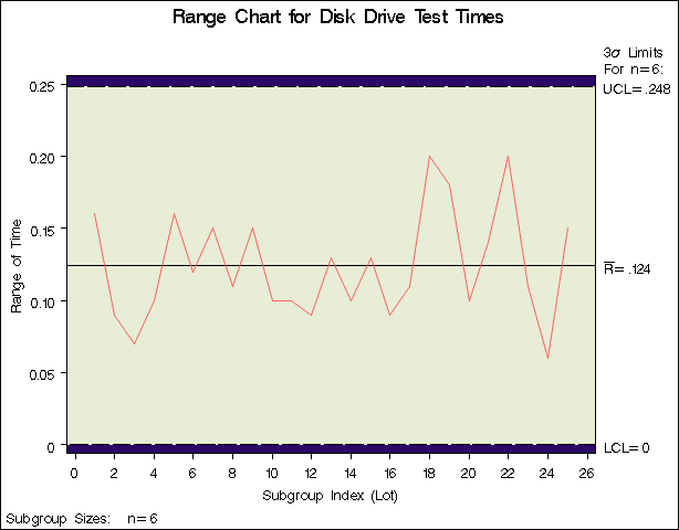
title 'Range Chart for Disk Drive Test Times';
proc shewhart history=Disksum;
rchart Time*Lot / cframe = vipb
cinfill = ywh
cconnect = rose;
run;
options gstyle;
The NOGSTYLE system option causes ODS styles not to affect traditional graphics. Instead, the SYMBOL statement and RCHART statement options control the appearance of the graph. The GSTYLE system option restores the use of ODS styles for traditional graphics produced subsequently. The resulting chart is shown in Figure 15.74.
Note that Time is not the name of a SAS variable in the data set Disksum but is, instead, the common prefix for the names of the SAS variables TimeR and TimeN. The suffix characters and  indicate range and sample size, respectively. Thus, you can specify two subgroup summary variables in the HISTORY= data set with a single name (Time), which is referred to as the process. The name Lot specified after the asterisk is the name of the subgroup-variable.
Chart from the Summary Data Set Disksum (Traditional Graphics with NOGSTYLE)
In general, a HISTORY= input data set used with the RCHART statement must contain the following variables:
subgroup variable
subgroup range variable
subgroup sample size variable
Furthermore, the names of the subgroup range and sample size variables must begin with the process name specified in the RCHART statement and end with the special suffix characters R and N, respectively. If the names do not follow this convention, you can use the RENAME optionin the PROC SHEWHART statement to rename the variables for the duration of the SHEWHART procedure step .
In summary, the interpretation of process depends on the input data set.
If raw data are read using the DATA= option (as in the previous example), process is the name of the SAS variable containing the process measurements.
If summary data are read using the HISTORY= option (as in this example), process is the common prefix for the names of the variables containing the summary statistics.
For more information, see HISTORY= Data Set.