PROC SHEWHART: OC Curve for Chart

Example 15.26 OC Curve for Chart

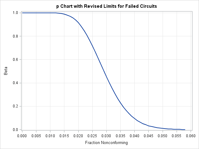
[See SHWPOC in the SAS/QC Sample Library]This example uses the GPLOT procedure and the OUTLIMITS= data set Faillim2 from the previous example to plot an OC curve for the $\text{[math]}$ chart shown in Output 15.25.3.

The OC curve displays $\text{[math]}$ (the probability that $\text{[math]}$ lies within the control limits) as a function of $\text{[math]}$ (the true proportion nonconforming). The computations are exact, assuming that the process is in control and that the number of nonconforming items ( $\text{[math]}$ ) has a binomial distribution.

The value of $\text{[math]}$ is computed as follows:

$\text{[math]}$	$\text{[math]}$	$\text{[math]}$
$\text{[math]}$	$\text{[math]}$	$\text{[math]}$
$\text{[math]}$	$\text{[math]}$	$\text{[math]}$
$\text{[math]}$	$\text{[math]}$	$\text{[math]}$
$\text{[math]}$	$\text{[math]}$	$\text{[math]}$

Here, $\text{[math]}$ denotes the incomplete beta function. The following DATA step computes $\text{[math]}$ (the variable BETA) as a function of $\text{[math]}$ (the variable P):

data ocpchart;
   set Faillim2;
   keep beta fraction _lclp_ _p_ _uclp_;
   nucl=_limitn_*_uclp_;
   nlcl=_limitn_*_lclp_;
   do p=0 to 500;
      fraction=p/1000;
      if nucl=floor(nucl) then
         adjust=probbnml(fraction,_limitn_,nucl) -
                probbnml(fraction,_limitn_,nucl-1);
      else adjust=0;
      if nlcl=0 then
         beta=1 - probbeta(fraction,nucl,_limitn_-nucl+1) + adjust;
      else beta=probbeta(fraction,nlcl,_limitn_-nlcl+1) -
                probbeta(fraction,nucl,_limitn_-nucl+1) +
                adjust;
      if beta >= 0.001 then output;
      end;
   call symput('lcl', put(_lclp_,5.3));
   call symput('mean',put(_p_,   5.3));
   call symput('ucl', put(_uclp_,5.3));
run;

The following statements display the OC curve shown in Output 15.26.1:

proc sgplot data=ocpchart;
   series x=fraction y=beta / lineattrs=(thickness=2);
   xaxis values=(0 to 0.06 by 0.005) grid;
   yaxis grid;
   label fraction = 'Fraction Nonconforming'
         beta     = 'Beta';
run;

Output 15.26.1 OC Curve for $\text{[math]}$ Chart

PCHART Statement: SHEWHART Procedure

Example 15.26 OC Curve for Chart