CCHART Statement: SHEWHART Procedure

Example 15.8 Applying Tests for Special Causes

[See SHWCEX1 in the SAS/QC Sample Library]This example illustrates how you can apply tests for special causes to make charts more sensitive to special causes of variation. Twenty trucks of the same model are inspected, and the number of paint defects per truck is recorded. The following statements create a SAS data set named Trucks3:

data Trucks3;
   input TruckID $ Defects @@;
   label TruckID='Truck Identification Number'
         Defects='Number of Paint Defects';
   datalines;
B1  12    B2  4    B3  4    B4   3
B5   4    D1  2    D2  3    D3   3
D4   2    D9  4    M2  9    M6  13
L3   5    L4  4    L7  6    Z1  15
Z2   8    Z3  9    Z7  6    Z9   8
;

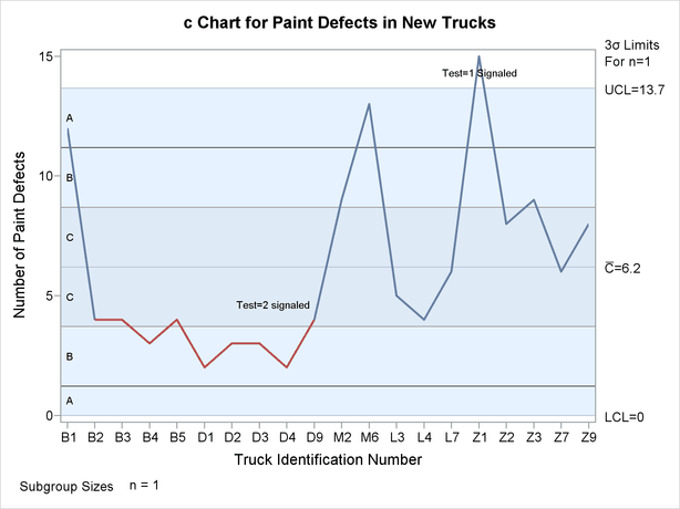
The following statements create a chart and tabulate the information on the chart. The chart and table are shown in Output 15.8.1 and Output 15.8.2.

ods graphics on;
title1 'c Chart for Paint Defects in New Trucks';
title2 'Tests=1 to 4';
proc shewhart data=Trucks3;
   cchart Defects*TruckID / tests      = 1 to 4
                            testlabel1 = 'Test=1 Signaled'
                            testlabel2 = 'Test=2 signaled'
                            odstitle   = title
                            zonelabels
                            tabletests
                            tablelegend;
run;

The TESTS= option requests Tests 1, 2, 3, and 4, which are described in Tests for Special Causes: SHEWHART Procedure. Only Tests 1, 2, 3, and 4 are recommended for charts. The TESTLABEL1= and TESTLABEL2= options specify the labels for points where Tests 1 and 2 are positive. The TESTFONT= option specifies the font for the labels indicating points at which the tests are positive.

Output 15.8.1 Tests for Special Causes Displayed on Chart

Output 15.8.2 Tabular Form of Chart

c Chart for Paint Defects in New Trucks

Tests=1 to 4

The SHEWHART Procedure

c Chart Summary for Defects
TruckID	Subgroup Sample Size	3 Sigma Limits with n=1 for Count			Special Tests Signaled
		Lower Limit	Subgroup Count	Upper Limit
B1	1.00000	0	12.000000	13.669940
B2	1.00000	0	4.000000	13.669940
B3	1.00000	0	4.000000	13.669940
B4	1.00000	0	3.000000	13.669940
B5	1.00000	0	4.000000	13.669940
D1	1.00000	0	2.000000	13.669940
D2	1.00000	0	3.000000	13.669940
D3	1.00000	0	3.000000	13.669940
D4	1.00000	0	2.000000	13.669940
D9	1.00000	0	4.000000	13.669940	2
M2	1.00000	0	9.000000	13.669940
M6	1.00000	0	13.000000	13.669940
L3	1.00000	0	5.000000	13.669940
L4	1.00000	0	4.000000	13.669940
L7	1.00000	0	6.000000	13.669940
Z1	1.00000	0	15.000000	13.669940	1
Z2	1.00000	0	8.000000	13.669940
Z3	1.00000	0	9.000000	13.669940
Z7	1.00000	0	6.000000	13.669940
Z9	1.00000	0	8.000000	13.669940

Test Descriptions
Test 1	One point beyond Zone A (outside control limits)
Test 2	Nine points in a row on one side of center line

The ZONELABELS option requests zone lines and displays zone labels on the chart. The zones are used to define the tests. The TABLETESTS option requests a table of counts of nonconformities, subgroup sample sizes, and control limits, together with a column indicating the subgroups at which the tests are positive. The TABLELEGEND option adds a legend describing the tests that are positive.

Output 15.8.1 and Output 15.8.2 indicate that Test 1 is positive at Truck Z1 and Test 2 is positive at Truck D9.