Example 11.3 Comparison of Univariate and Multivariate Control Charts
This example shows the effect of a change in correlation of the process variables on the SPE chart. The following statements create a data set that consists of 30 samples from a trivariate normal distribution with strong positive correlation between all three variables:
proc iml;
   Mean = {0,0,0};
   Cor = {1.0 0.8 0.8,
          0.8 1.0 0.8,
          0.8 0.8 1.0};
   StdDevs = {2 2 2};
   D = diag(StdDevs);
   Cov = D*Cor*D; /* covariance matrix */
   NumSamples = 30;
   call randseed(123321);  /* set seed for the RandNormal module */
   X = RandNormal(NumSamples, Mean, Cov);
   varnames = { x1 x2 x3};
   create mvpStable from X [colname = varnames];
   append from X;
   quit;
run;
data mvpStable;
   set mvpStable;
   hour=_n_;
run;
The next statements create a data set with five observations in which the correlations are negative:
proc iml;
   Mean = {0,0,0};
   Cor = { 1.0 -0.8  0.8,
          -0.8  1.0 -0.8,
           0.8 -0.8  1.0};
   StdDevs = {2 2 2};
   D = diag(StdDevs);
   Cov = D*Cor*D; /* covariance matrix */
   NumSamples = 5;
   call randseed(123321);  /* set seed for the RandNormal module */
   X = RandNormal(NumSamples, Mean, Cov);
   varnames = { x1 x2 x3};
   create mvpOOC from X [colname = varnames];
   append from X;
   quit;
run;
data mvpOOC;
   set mvpStable mvpOOC;
   hour=_n_;
run;
The following statements produce a principal components model for the data in mvpStable:
proc mvpmodel data=mvpStable ncomp=1 plots=none out=scores
              outloadings=loadings timegroup= hour;
   var x1 x2 x3;
run;
The model hyperplane defined by the NCOMP= option is a line. The loadings in the principal components model, which are used to project the data to the model hyperplane, are defined by the correlation structure present in the DATA= data set.
The model explains about 90% of the variance in the data as shown in Output 11.3.1.
| Eigenvalues of the Correlation Matrix | ||||
|---|---|---|---|---|
| Eigenvalue | Difference | Proportion | Cumulative | |
| 1 | 2.67725690 | 0.8924 | 0.8924 | |
The loadings from the model are then applied to the data in mvpOOC, which includes observations with a different correlation structure, which vary in direction orthogonal to the model line.
proc mvpmonitor data=mvpOOC loadings=loadings;
   time hour;
   scoreplot;
   tsquarechart;
   spechart;
run;
The MVPMONITOR procedure generates a  chart, shown in Output 11.3.2.
Chart
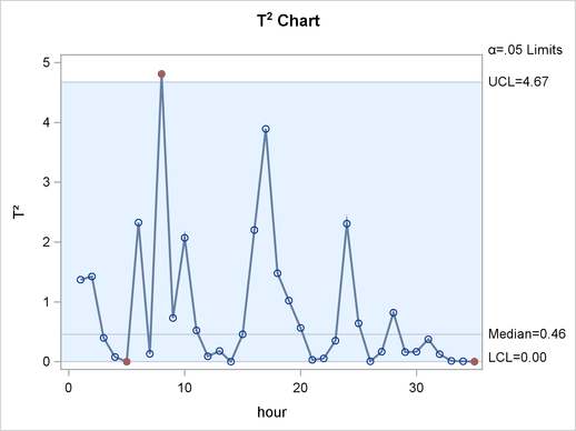
The projection of the last five points to the model line results in small amounts of variation, and thus small statistics because of two reasons—the last five points are orthogonal to the model line, and they share the same mean. However, the orthogonality means that they are out-of-control points on the SPE chart.
The MVPMONITOR procedure also produces an SPE chart, Output 11.3.3.
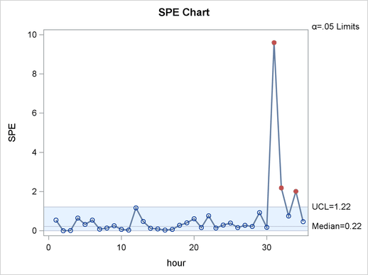
Since the last five points come from a correlation structure that is not seen in the data from which the model was built, they can lie far from the model line, resulting in large values in the SPE statistics.
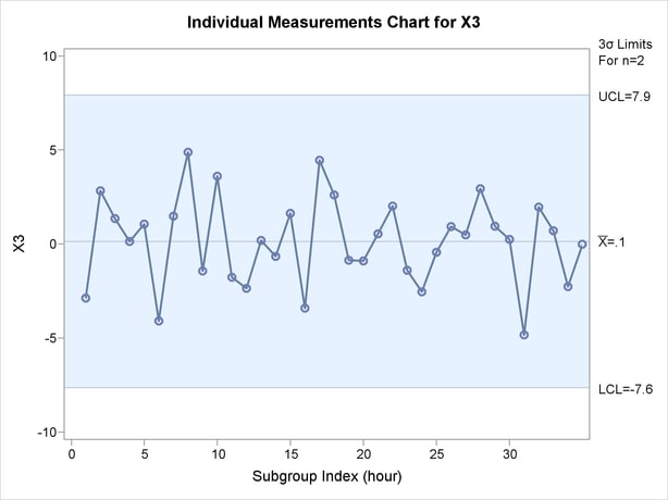
Since the marginal distributions are the same in both the original 30 points and the additional five points, the univariate control charts in Output 11.3.4, Output 11.3.5, and Output 11.3.6 fail to signal the multivariate change at hour 31.
proc shewhart data=mvpOOC;
   irchart (x1 x2 x3) * hour / markers nochart2;
run;

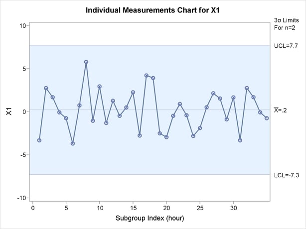

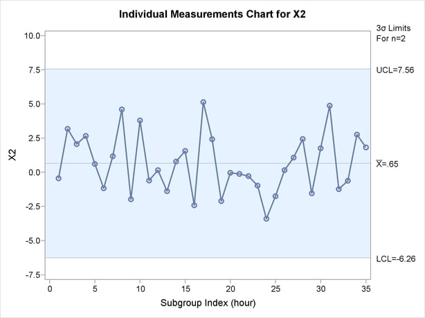

Note: This procedure is experimental.