Calculating Probability Limits

The OUTLIMITS= option saves the control limits from the chart in Figure 13.43.98 in a SAS data set named DELAYLIM, which is listed in Figure 13.43.99.

The control limits can be replaced with the corresponding percentiles from a fitted lognormal distribution. The equation for the lognormal density function is

where denotes the shape parameter and denotes the scale parameter.

The following statements use the CAPABILITY procedure to fit a lognormal model and superimpose the fitted density on a histogram of the data, shown in Figure 13.43.100:

title 'Lognormal Fit for Delay Distribution';
proc capability data=Calls noprint;
   histogram Time /
      lognormal(threshold=2.3 w=2)
      outfit = Lnfit
      nolegend ;
   inset n = 'Number of Calls'
      lognormal( sigma = 'Shape' (4.2)
                 zeta  = 'Scale' (5.2)
                 theta ) / pos    = ne;
   label Time  = 'Answering Delay (minutes)';
run;

Output 13.43.100 Distribution of Delays

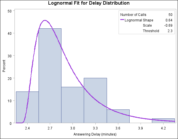
Parameters of the fitted distribution and results of goodness-of-fit tests are saved in the data set LNFIT, which is listed in Figure 13.43.101. The large -values for the goodness-of-fit tests are evidence that the lognormal model provides a good fit.

The following statements replace the control limits in DELAYLIM with limits computed from percentiles of the fitted lognormal model. The 100th percentile of the lognormal distribution is 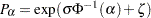, where denotes the inverse standard normal cumulative distribution function. The SHEWHART procedure constructs an chart with the modified limits, displayed in Figure 13.43.102.

data delaylim;
   merge delaylim Lnfit;
   drop _sigmas_ ;
   _lcli_ = _locatn_ + exp(_scale_+probit(0.5*_alpha_)*_shape1_);
   _ucli_ = _locatn_ + exp(_scale_+probit(1-.5*_alpha_)*_shape1_);
   _mean_ = _locatn_ + exp(_scale_+0.5*_shape1_*_shape1_);
run;

title 'Lognormal Control Limits for Delays';
proc shewhart data=Calls limits=delaylim;
   irchart Time*Recnum /
      rtmplot   = schematic
      nochart2 ;
   label Recnum = 'Record Number'
         Time   = 'Delay in minutes' ;
run;

Output 13.43.102 Adjusted Control Limits for Delays

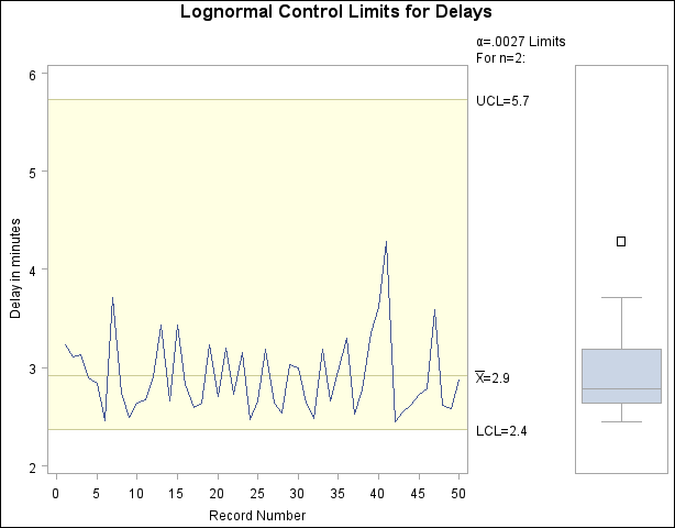
Clearly the process is in control, and the control limits (particularly the lower limit) are appropriate for the data. The particular probability level associated with these limits is somewhat immaterial, and other values of such as 0.001 or 0.01 could be specified with the ALPHA= option in the original IRCHART statement.