| The SHEWHART Procedure |
Strategies for Handling Autocorrelation
There is considerable disagreement on how to handle autocorrelation in process data. Consider the following three views:
At one extreme, Wheeler (1991) argues that the usual control limits are contaminated "only when the autocorrelation becomes excessive (say 0.80 or larger)." He concludes that "one need not be overly concerned about the effects of autocorrelation upon the control chart."
At the opposite extreme, automatic process control (APC), also referred to as engineering process control, views autocorrelation as a phenomenon to be exploited. In contrast to SPC, which assumes that the process remains on target unless an unexpected but removable cause occurs, APC assumes that the process is changing dynamically due to known causes that cannot be eliminated. Instead of avoiding "overcontrol" and "tampering," which have a negative connotation in the SPC framework, APC advocates continuous tuning of the process to achieve minimum variance control. Descriptions of this approach and discussion of the differences between APC and SPC are provided by a number of authors, including Box and Kramer (1992), MacGregor (1987, 1990), MacGregor, Hunter, and Harris (1988), and Montgomery et al. (1994).
A third strategy advocates removing autocorrelation from the data and constructing a Shewhart chart (or an EWMA chart or a cusum chart) for the residuals; refer, for example, to Alwan and Roberts (1988).
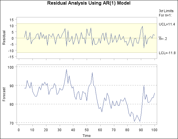
An example of the last approach is presented in the remainder of this section simply to demonstrate the use of the ARIMA procedure in conjunction with the SHEWHART procedure. The ARIMA procedure models the autocorrelation and saves the residuals in an output data set; the SHEWHART procedure creates a control chart using the residuals as input data.
In the chemical data example, the residuals can be computed as forecast errors and saved in an output SAS data set with the FORECAST statement in the ARIMA procedure.
proc arima data=Chemical;
   identify var=xt;
   estimate p=1 method=ml;
   forecast out=Results id=t;
run;
The output data set (named Results) saves the one-step-ahead forecasts as a variable named FORECAST, and it also contains the original variables xt and t. You can create a Shewhart chart for the residuals by using the data set Results as input to the SHEWHART procedure.
title 'Residual Analysis Using AR(1) Model';
symbol h=2.0 pct;
proc shewhart data=Results(firstobs=4 obs=100);
   xchart xt*t / npanelpos = 100
                 split     = '/'
                 trendvar  = forecast
                 xsymbol   = xbar
                 ypct1     = 40
                 vref2     = 70 to 100 by 10
                 lvref     = 2
                 nolegend;
   label xt = 'Residual/Forecast'
          t = 'Time';
run;
The chart is shown in Figure 13.43.77. Specifying TRENDVAR=FORECAST plots the values of FORECAST in the lower chart and plots the residuals (xt  FORECAST) together with their
  limits in the upper chart.1
Various other methods can be applied with this data. For example, Montgomery and Mastrangelo (1991) suggest fitting an exponentially weighted moving average (EWMA) model and using this model as the basis for a display that they refer to as an EWMA central line control chart.
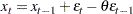
Before presenting the statements for creating this display, it is helpful to review some terminology. The EWMA statistic plotted on a conventional EWMA control chart is defined as
 |
The EWMA chart (which you can construct with the MACONTROL procedure) is based on the assumption that the observations  are independent. However, in the context of autocorrelated process data (and more generally in time series analysis), the EWMA statistic
  plays a different role:2 it is the optimal one-step-ahead forecast for a process that can be modeled by an ARIMA(0,1,1) model
 |
provided that the weight parameter  is chosen as
  . This statistic is also a good predictor when the process can be described by a subset of ARIMA models for which the process is "positively autocorrelated and the process mean does not drift too quickly."3
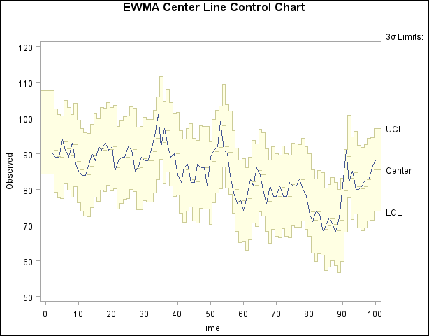
You can fit an ARIMA(0,1,1) model to the chemical data with the following statements. A summary of the fitted model is shown in Figure 13.43.78.
title ;
proc arima data=Chemical;
   identify var=xt(1);
   estimate q=1 method=ml noint;
   forecast out=EWMA id=t;
run;
| Maximum Likelihood Estimation | |||||
|---|---|---|---|---|---|
| Parameter | Estimate | Standard Error | t Value | Approx Pr > |t| |
Lag |
| MA1,1 | 0.15041 | 0.10021 | 1.50 | 0.1334 | 1 |
The forecast values and their standard errors (variables FORECAST and STD), together with the original measurements, are saved in a data set named EWMA. The EWMA central line control chart plots the forecasts from the ARIMA(0,1,1) model as the central "line," and it uses the standard errors of prediction to determine upper and lower control limits. You can construct this chart, shown in Figure 13.43.79,4 with the following statements:
data EWMA;
   set EWMA(firstobs=2 obs=100);
run;

data EWMAtab;
   length _var_ $ 8 ;
   set EWMA (rename=(forecast=_mean_ xt=_subx_));
   _var_    = 'xt';
   _sigmas_ = 3;
   _limitn_ = 1;
   _lclx_   = _mean_ - 3 * std;
   _uclx_   = _mean_ + 3 * std;
   _subn_   = 1;
run;
symbol h=2.0 pct;
title 'EWMA Center Line Control Chart';
proc shewhart table=EWMAtab;
   xchart xt*t / npanelpos = 100
                 xsymbol   = 'Center'
                 nolegend;
   label _subx_ = 'Observed'
              t = 'Time' ;
run;
Note that EWMA is read by the SHEWHART procedure as a TABLE= input data set, which has a special structure intended for applications in which both the statistics to be plotted and their control limits are pre-computed. The variables in a TABLE= data set have reserved names beginning and ending with the underscore character; for this reason, FORECAST and xt are temporarily renamed as _MEAN_ and _SUBX_, respectively. For more information about TABLE= data sets, see "Input Data Sets" in the section for the chart statement in which you are interested.
Again, the conclusion is that the process is in control. While Figure 13.43.77 and Figure 13.43.79 are not the only displays that can be considered for analyzing the chemical data, their construction illustrates the conjunctive use of the ARIMA and SHEWHART procedures in process control applications involving autocorrelated data.
Footnotes
- The upper chart in Figure 13.43.77 resembles Figure 2 of Montgomery and Mastrangelo (1991), who conclude that the process is in control.
- For a discussion of these roles, refer to Hunter (1986).
- Refer to Montgomery and Mastrangelo (1991) and the discussion that follows their paper.
- Figure 13.43.79 is similar to Figure 5 of Montgomery and Mastrangelo (1991).
Copyright © SAS Institute, Inc. All Rights Reserved.