| The RELIABILITY Procedure |
| Recurrence Data from Repairable Systems |
When a repairable system fails, it is repaired and placed back in service. As a repairable system ages, it accumulates a history of repairs and costs of repairs. The mean cumulative function (MCF)  is defined as the population mean of the cumulative number (or cost) of repairs up until time
  . You can use the RELIABILITY procedure to compute and plot nonparametric estimates and plots of the MCF for the number of repairs or the cost of repairs. The Nelson (1995) confidence limits for the MCF are also computed and plotted. You can compute and plot estimates of the difference of two MCFs and confidence intervals. This is useful for comparing the repair performance of two systems.
See Nelson (2002, 1995, 1988) , Doganaksoy and Nelson (1998) , and Nelson and Doganaksoy (1989) for discussions and examples of analysis of recurrence data.
Recurrence Data with Exact Ages
See the section Analysis of Recurrence Data on Repairs and the section Comparison of Two Samples of Repair Data for examples of the analysis of recurrence data with exact ages.
Formulas for the MCF estimator  and the variance of the estimator Var
 are given in Nelson (1995). Table 12.61 shows a set of artificial repair data from Nelson (1988). For each system, the data consist of the system and cost for each repair. If you want to compute the MCF for the number of repairs, rather than cost of repairs, then you should set the cost equal to 1 for each repair. A plus sign (+) in place of a cost indicates that the age is a censoring time. The repair history of each system ends with a censoring time.
Unit |
(Age in Months, Cost in $100) |
|||
|---|---|---|---|---|
6 |
(5,$3) |
(12,$1) |
(12,+) |
|
5 |
(16,+) |
|||
4 |
(2,$1) |
(8,$1) |
(16,$2) |
(20,+) |
3 |
(18,$3) |
(29,+) |
||
2 |
(8,$2) |
(14,$1) |
(26,$1) |
(33,+) |
1 |
(19,$2) |
(39,$2) |
(42,+) |
|
Table 12.62 illustrates the calculation of the MCF estimate from the data in Table 12.61. The RELIABILITY procedure uses the following rules for computing the MCF estimates.
Order all events (repairs and censoring) by age from smallest to largest.
If the event ages of the same or different systems are equal, the corresponding data are sorted from the largest repair cost to the smallest. Censoring events always sort as smaller than repair events with equal ages.
When event ages and values of more than one system coincide, the corresponding data are sorted from the largest system identifier to the smallest. The system IDs can be numeric or character, but they are always sorted in ASCII order.
Compute the number of systems
 in service at the current age as the number in service at the last repair time minus the number of censored units in the intervening times.
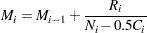
 For each repair, compute the mean cost as the cost of the current repair divided by the number in service
. Compute the MCF for each repair as the previous MCF plus the mean cost for the current repair.
Number |
Mean |
|||
|---|---|---|---|---|
Event |
(Age,Cost) |
Service |
Cost |
MCF |
1 |
(2,$1) |
6 |
$1/6=0.17 |
0.17 |
2 |
(5,$3) |
6 |
$3/6=0.50 |
0.67 |
3 |
(8,$2) |
6 |
$2/6=0.33 |
1.00 |
4 |
(8,$1) |
6 |
$1/6=0.17 |
1.17 |
5 |
(12,$1) |
6 |
$1/6=0.17 |
1.33 |
6 |
(12,+) |
5 |
||
7 |
(14,$1) |
5 |
$1/5=0.20 |
1.53 |
8 |
(16,$2) |
5 |
$2/5=0.40 |
1.93 |
9 |
(16,+) |
4 |
||
10 |
(18,$3) |
4 |
$3/4=0.75 |
2.68 |
11 |
(19,$2) |
4 |
$2/4=0.50 |
3.18 |
12 |
(20,+) |
3 |
||
13 |
(26,$1) |
3 |
$1/3=0.33 |
3.52 |
14 |
(29,+) |
2 |
||
15 |
(33,+) |
1 |
||
16 |
(39,$2) |
1 |
$2/1=2.00 |
5.52 |
17 |
(42,+) |
0 |
The variance of the estimator of the MCF Var is computed as in Nelson (1995). If the VARIANCE=LAWLESS or VARMETHOD2 option is specified, the method of Lawless and Nadeau (1995) is used to compute the variance of the estimator of the MCF. This method is recommended if the number of systems or events is large or if a FREQ statement is used to specify a frequency variable.
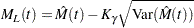
Default approximate two-sided  pointwise confidence limits for are computed as
 |
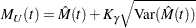 |
where  represents the
  percentile of the standard normal distribution.
If you specify the LOGINTERVALS option in the MCFPLOT statement, alternative confidence intervals based on the asymptotic normality of  , rather than of , are computed. Let
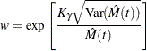 |
Then the limits are computed as
 |
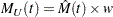 |
These alternative limits are always positive, and can provide better coverage than the default limits when the MCF is known to be positive, such as for counts or for positive costs. They are not appropriate for MCF differences, and are not computed in this case.
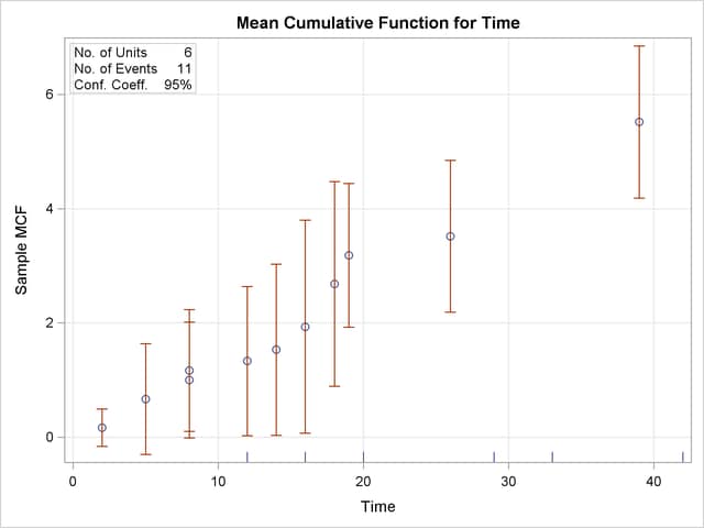
The following SAS statements create the tabular output shown in Figure 12.47 and the plot shown in Figure 12.48:
   data Art;
      input Sysid$ Time Cost;
      datalines;
      sys1 19 2
      sys1 39 2
      sys1 42 -1
      sys2 8  2
      sys2 14 1
      sys2 26 1
      sys2 33 -1
      sys3 18 3
      sys3 29 -1
      sys4 16 2
      sys4 2  1
      sys4 20  -1
      sys4 8  1
      sys5 16 -1
      sys6 5 3
      sys6 12 1
      sys6 12 -1
      ;
   run;
proc reliability data=Art;
   unitid Sysid;
   mcfplot Time*Cost(-1) ;
run;
The first table in Figure 12.47 displays the input data set, the number of observations used in the analysis, the number of systems (units), and the number of repair events. The second table displays the system age, MCF estimate, standard error, approximate confidence limits, and system ID for each event.
| Recurrence Data Summary | |
|---|---|
| Input Data Set | WORK.ART |
| Observations Used | 17 |
| Number of Units | 6 |
| Number of Events | 11 |
| Recurrence Data Analysis | |||||
|---|---|---|---|---|---|
| Age | Sample MCF | Standard Error | 95% Confidence Limits | Unit ID | |
| Lower | Upper | ||||
| 2.00 | 0.167 | 0.167 | -0.160 | 0.493 | sys4 |
| 5.00 | 0.667 | 0.494 | -0.302 | 1.636 | sys6 |
| 8.00 | 1.000 | 0.516 | -0.012 | 2.012 | sys2 |
| 8.00 | 1.167 | 0.543 | 0.103 | 2.230 | sys4 |
| 12.00 | 1.333 | 0.667 | 0.027 | 2.640 | sys6 |
| 12.00 | . | . | . | . | sys6 |
| 14.00 | 1.533 | 0.764 | 0.035 | 3.032 | sys2 |
| 16.00 | 1.933 | 0.951 | 0.069 | 3.797 | sys4 |
| 16.00 | . | . | . | . | sys5 |
| 18.00 | 2.683 | 0.913 | 0.894 | 4.473 | sys3 |
| 19.00 | 3.183 | 0.641 | 1.926 | 4.440 | sys1 |
| 20.00 | . | . | . | . | sys4 |
| 26.00 | 3.517 | 0.679 | 2.185 | 4.848 | sys2 |
| 29.00 | . | . | . | . | sys3 |
| 33.00 | . | . | . | . | sys2 |
| 39.00 | 5.517 | 0.679 | 4.185 | 6.848 | sys1 |
| 42.00 | . | . | . | . | sys1 |
Estimates of the difference between two MCFs  and the variance of the estimator are computed as in Doganaksoy and Nelson (1998). Confidence limits for the MCF difference function are computed in the same way as for the MCF, by using the variance of the MCF difference function estimator.
Recurrence Data with Ages Grouped into Intervals
Recurrence data are sometimes grouped into time intervals for convenience, or to reduce the number of data records to be stored and analyzed. Interval recurrence data consist of the number of recurrences and the number of censored units in each time interval.
You can use PROC RELIABILITY to compute and plot MCFs and MCF differences for interval data. Formulas for the MCF estimator and the variance of the estimator Var for interval data, as well as examples and interpretations, are given in Nelson (2002, chapter 5). These calculations apply only to the number of recurrences, and not to cost.
Let  be the total number of units,
  the number of recurrences in interval
  ,
,  , and
, and  the number of units censored into interval . Then
  and the number entering interval is
 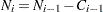 with
with  . The MCF estimate for interval is
  ,
,
 |
The denominator  approximates the number at risk in interval , and treats the censored units as if they were censored halfway through the interval. Since no censored units are likely to have ages lasting through the entire last interval, the MCF estimate for the last interval is likely to be biased. A footnote is printed in the tabular output as a reminder of this bias for the last interval.
See the section Analysis of Interval Age Recurrence Data for an example of interval recurrence data analysis.
Copyright © SAS Institute, Inc. All Rights Reserved.