| The RELIABILITY Procedure |
| Analysis of Right-Censored Data from a Single Population |
The Weibull distribution is used in a wide variety of reliability analysis applications. This example illustrates the use of the Weibull distribution to model product life data from a single population. The following statements create a SAS data set containing observed and right-censored lifetimes of 70 diesel engine fans (Nelson; 1982, p. 318) :
   data fan;
      input lifetime censor @@;
      lifetime = lifetime/1000;
      label lifetime='Fan Life (1000s of Hours)';
      datalines;
       450 0    460 1   1150 0   1150 0   1560 1
      1600 0   1660 1   1850 1   1850 1   1850 1
      1850 1   1850 1   2030 1   2030 1   2030 1
      2070 0   2070 0   2080 0   2200 1   3000 1
      3000 1   3000 1   3000 1   3100 0   3200 1
      3450 0   3750 1   3750 1   4150 1   4150 1
      4150 1   4150 1   4300 1   4300 1   4300 1
      4300 1   4600 0   4850 1   4850 1   4850 1
      4850 1   5000 1   5000 1   5000 1   6100 1
      6100 0   6100 1   6100 1   6300 1   6450 1
      6450 1   6700 1   7450 1   7800 1   7800 1
      8100 1   8100 1   8200 1   8500 1   8500 1
      8500 1   8750 1   8750 0   8750 1   9400 1
      9900 1  10100 1  10100 1  10100 1  11500 1
      ;
   run;
Some of the fans had not failed at the time the data were collected, and the unfailed units have right-censored lifetimes. The variable Lifetime represents either a failure time or a censoring time in thousands of hours. The variable Censor is equal to 0 if the value of Lifetime is a failure time, and it is equal to 1 if the value is a censoring time.
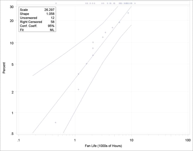
The following statements use the RELIABILITY procedure to produce the graphical output shown in Figure 12.1:
proc reliability data=fan;
   distribution weibull;
   pplot lifetime*censor( 1 ) /  covb ;
run;
The DISTRIBUTION statement specifies the Weibull distribution for probability plotting and maximum likelihood (ML) parameter estimation. The PROBPLOT statement produces a probability plot for the variable Lifetime and specifies that the value of 1 for the variable Censor denotes censored observations. You can specify any value, or group of values, for the censor-variable (in this case, Censor) to indicate censoring times. The option COVB requests the ML parameter estimate covariance matrix.
The graphical output, displayed in Figure 12.1, consists of a probability plot of the data, an ML fitted distribution line, and confidence intervals for the percentile (lifetime) values. An inset box containing summary statistics, Weibull scale and shape estimates, and other information is displayed on the plot by default. The locations of the right-censored data values are plotted in an area at the top of the plot.

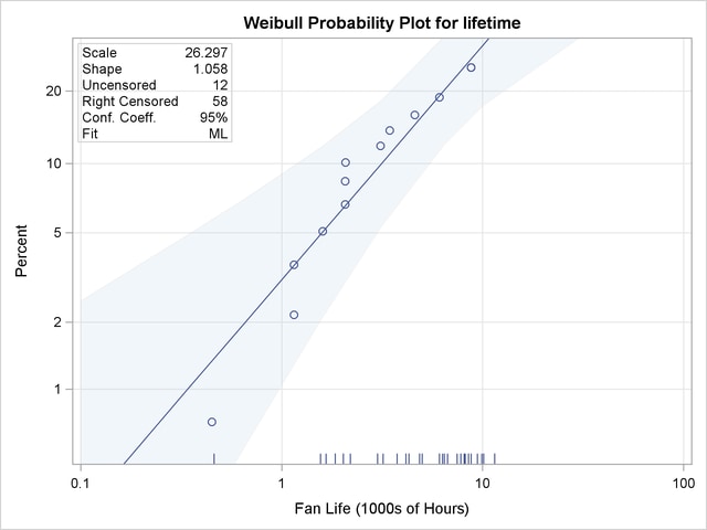
You can optionally create the probability plot by using ODS Graphics. The following SAS statements use ODS Graphics to create the probability plot shown in Figure 12.1:
ods graphics ON;
proc reliability data=fan;
   distribution weibull;
   pplot lifetime*censor( 1 ) /  covb;
run;
ods graphics OFF;
The plot is shown in Figure 12.2.

The tabular output produced by the preceding SAS statements is shown in Figure 12.3 and Figure 12.4. This consists of summary data, fit information, parameter estimates, distribution percentile estimates, standard errors, and confidence intervals for all estimated quantities.
| Model Information | ||
|---|---|---|
| Input Data Set | WORK.FAN | |
| Analysis Variable | lifetime | Fan Life (1000s of Hours) |
| Censor Variable | censor | |
| Distribution | Weibull | |
| Estimation Method | Maximum Likelihood | |
| Confidence Coefficient | 95% | |
| Observations Used | 70 | |
| Summary of Fit | |
|---|---|
| Observations Used | 70 |
| Uncensored Values | 12 |
| Right Censored Values | 58 |
| Maximum Loglikelihood | -42.248 |
| Weibull Parameter Estimates | ||||
|---|---|---|---|---|
| Parameter | Estimate | Standard Error | Asymptotic Normal | |
| 95% Confidence Limits | ||||
| Lower | Upper | |||
| EV Location | 3.2694 | 0.4659 | 2.3563 | 4.1826 |
| EV Scale | 0.9448 | 0.2394 | 0.5749 | 1.5526 |
| Weibull Scale | 26.2968 | 12.2514 | 10.5521 | 65.5344 |
| Weibull Shape | 1.0584 | 0.2683 | 0.6441 | 1.7394 |
| Other Weibull Distribution Parameters | |
|---|---|
| Parameter | Value |
| Mean | 25.7156 |
| Mode | 1.7039 |
| Median | 18.6002 |
| Standard Deviation | 24.3066 |
| Weibull Percentile Estimates | ||||
|---|---|---|---|---|
| Percent | Estimate | Standard Error | Asymptotic Normal | |
| 95% Confidence Limits | ||||
| Lower | Upper | |||
| 0.1 | 0.03852697 | 0.05027782 | 0.002985 | 0.49726229 |
| 0.2 | 0.07419554 | 0.08481353 | 0.00789519 | 0.69725757 |
| 0.5 | 0.17658807 | 0.16443381 | 0.02846732 | 1.09540855 |
| 1 | 0.34072273 | 0.2635302 | 0.07482449 | 1.55152389 |
| 2 | 0.65900116 | 0.40845639 | 0.19556981 | 2.22060107 |
| 5 | 1.58925244 | 0.68465855 | 0.68311002 | 3.69738878 |
| 10 | 3.13724079 | 0.99379006 | 1.68620756 | 5.83693255 |
| 20 | 6.37467675 | 1.74261908 | 3.73051433 | 10.8930029 |
| 30 | 9.92885165 | 3.00353842 | 5.48788931 | 17.9635721 |
| 40 | 13.9407124 | 4.85766683 | 7.04177638 | 27.5986417 |
| 50 | 18.6002319 | 7.40416922 | 8.52475116 | 40.5840149 |
| 60 | 24.2121441 | 10.8733301 | 10.0408557 | 58.3842593 |
| 70 | 31.3378076 | 15.750336 | 11.7018888 | 83.9230489 |
| 80 | 41.2254517 | 23.1787018 | 13.6956839 | 124.092954 |
| 90 | 57.8253251 | 36.9266698 | 16.5405275 | 202.156081 |
| 95 | 74.1471722 | 51.6127806 | 18.9489625 | 290.137423 |
| 99 | 111.307797 | 88.1380261 | 23.5781482 | 525.462197 |
| 99.9 | 163.265082 | 144.264145 | 28.8905203 | 922.637827 |
Copyright © SAS Institute, Inc. All Rights Reserved.